Live Optics | Optical Prime | VMware Guest VM Performance

The concepts in this document are not only important to proper collections and sizing. They are critical to understanding the importance of cost as it pertains to the Public Cloud vs. a Private Cloud. These concepts are discussed in more detail at the closing of this document.

Hypervisor Performance

Hypervisor performance is gathered "Live," hence the naming of Live Optics. This is a capture of performance metrics from the moment that you start the collection until the end of the duration you selected.

This means that Live Optics polls vCenter and creates telemetry files in real-time.

VM Performance

Guest VM Performance data can be optionally selected, but it is enabled by default.

VMware provides access to the individual Virtual Machine data through an archive telemetry file.

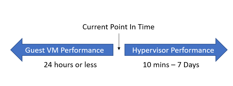
Guest VM Performance telemetry files are not consistent in an environment. The VMware admin can configure the archives, per metric, to hold telemetry data for minutes, hours or longer. So, while Live Optics can pull this data, the data might vary per metric or per environment.

In its current form, Optical Prime takes these archive metrics for IOPS, Memory, CPU, so forth, and creates data points, like "Peak IOPS." These calculated metrics are posted to the VM details in the Excel output from the portal.

VM Performance telemetry retrieval does create an increased burden on the collection. Depending on the environment, it can take between 1 s and 5 s per VM to complete this retrieval.

This creates little overhead on the collection environment, but it takes time and Optical Prime must ensure that this time is compensated for in the runtime of the executable.

Using some basic math, if 50,000 VMs took the worst-case scenario of 5 s per VM, there would be a minimum of roughly a 3-day waiting period to retrieve all this data.

For that reason, the collection of Guest VM performance data is bound to Optical Prime’s performance collection routines and the collector prohibits the selection of a recording duration that is below the estimated retrieval time for all VM telemetry files.

In the above scenario, the minimum collection duration to record performance would be at least 3 days.

Understanding Performance Data

When you are looking to understand an environment’s performance, you should be using the Hypervisor’s performance data.

Depending on the approach taken, using Guest VM performance data found in the Excel sheet could lead to dramatically overestimating performance needs.

To understand this, let me deep dive in the mechanics of how all this works.

When "DPACK," the founding name of Live Optics, came into the market it was solving a fundamental misunderstanding in the industry.

This misunderstanding was perpetuated for years due to the complexity of performing these tasks correctly. It takes software to do it right, it is a big data problem and Live Optics has commoditized this for the industry.

This fallible approach in the industry was called "adding the peaks" and there is definitive proof that it is a misleading approach to sizing projects. Let me explain in a simplified, but fabricated scenario.

Example 1:

Server A does 500 IOPS at peak and Server B does 500 IOPS at peak, the logical assumption is that you need 1,000 IOPS to accommodate both machines.

This method is called the "Adding The Peaks" methodology. It was derived due to the complexity of aggregating 'data' over 'time.'

Windows has Perfmon data, Linux has IOSTAT, and back in the day people focused on ESXTOP for performance data from VMware environments.

Communities found it difficult to associate files of unlike formats correctly, so the only options were to either guess at requirements or add up the peaks.

Example 2:

Now let us repeat the exercise but give you more data points. Server As peak occurs at 3 PM and Server B’s peak occurs at 4 PM.

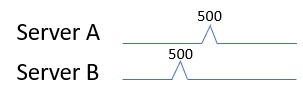
The Live Optics collector initiates the collection of data simultaneously to all end points for which it records data. It also does so in a proprietary format so that all data points can be aligned perfectly to form an "Aggregated" view of performance.

For this basic example, let us assume this is the ONLY activity that these servers produced throughout the day. Once you consider that Server A and Server B’s activity does not occur simultaneously, we can clearly see that we do not need 1,000 IOPS at all. We only need 500 IOPS.

This method is called the "Time Aligned Aggregation" method, and it is the method that Live Optics pioneered and then commoditized for the Industry.

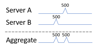
Example 3:

Obviously, there are not servers in the world that only do activity for a moment and then sit dormant the rest of the day. Let us expand this figure to show how this works at scale.

"Adding the Peaks" will be illustrated by the Red/Dashed lines.
"Time Aligned Aggregation" will be is illustrated by the Green/Solid lines.

Server performance in respect to IOPS is a "per second" metric by definition: I/Os Per Second. IOPS are also volatile throughout the day as the server shifts between cycles of "thinking" and "executing."

This means that the simplified scenario of Example 2 is played out thousands of times a day and it means that the more servers you have participating the greater the variance will be between the two methodologies.

In other words, the more servers that are participating, the more inaccurate the "Adding the Peaks" methodology becomes.

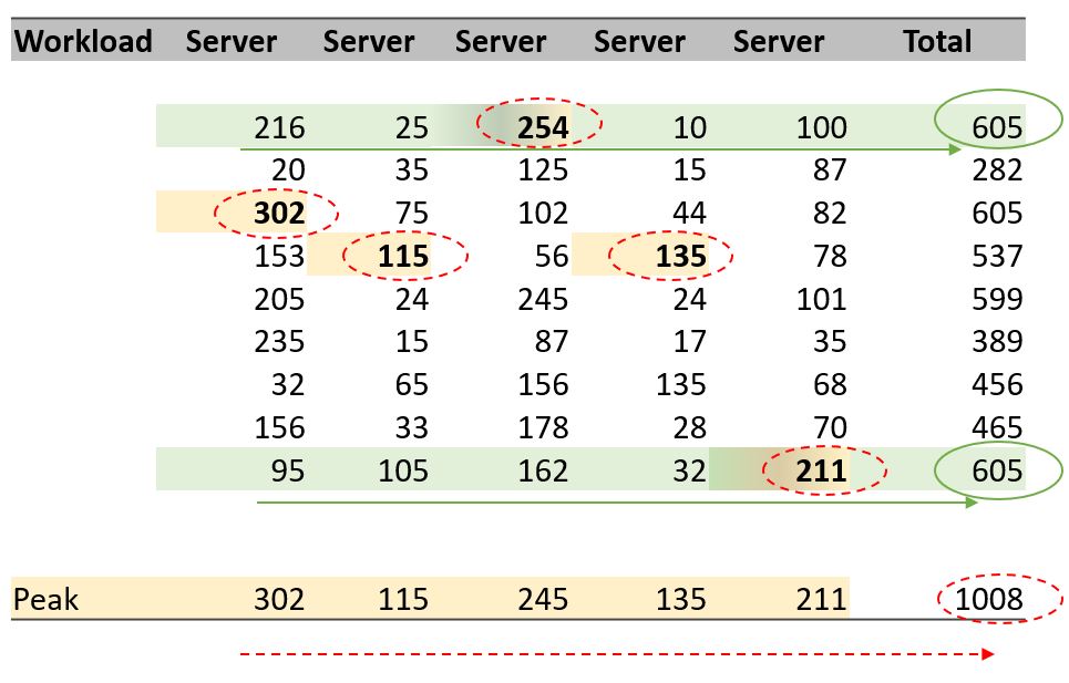
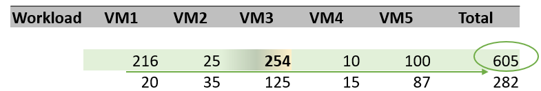
We can see in the figure below, that if we added the peak activity of all these VMs they would lead to a near 40% overcompensation to the true requirements of only 605.

When all servers at any given time were operating, they never exceeded 605 IOPS.  

Example 4:

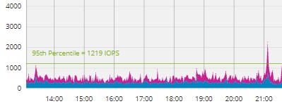
Since any scenario can be manufactured to illustrate a point, let us look at an actual project.

This project contains 344 running VMs. If I exported the Excel output for this project, I would get all the Peak IOPS metrics for each of these Virtual Machines.

Excel makes it to SUM() the IOPS values and the result is 4,454 IOPS.

Alternately, the Time-Aligned Aggregation allows us to create a 95^th percentile over the entire dataset and evaluate the blended performance of all these machines.

The answer is dramatically different, and the computed results are only 1,219 IOPS, a value 73% lower compared to adding up the peaks. 

Results

This is critical for determining project sizing and to understand that this same effect will occur for IOPS, memory, CPU, throughput, and network traffic.

However, this will not impact capacity sizing. Capacity is not measured over time and would not be volatile enough to make any real difference in project requirements.

When it comes to size any shared resource environment like Hyperconverged, VSAN or even a shared external storage array, this is essential data that must be considered.

One can see this substantially lowers the entry point for project requirements but does so in a far superior manner using powerful software in the Live Optics portal to simplify this task.

Live Optics computes all these values for you, and since the values are abstracted from the hardware powering the workload, you can create effective simulations of mixed platforms and Operating Systems under "what if" scenarios.

Why it works

There is a large philosophical debate as to what metrics should be used for sizing. The schools of thought are: from the VMs, from the Hypervisor, or from the storage array.

In this illustration, we break this down.

For background, Live Optics standardizes on Front End IOPS. The term "Front End" is seeing the IOPS that are originated by the application or the Operating System. These are platform and vendor agnostic as opposed to the Back End IOPS that will be technology- and vendor-specific.

A quick example: if a server has 15 Front End write IOPS and the data is written in a RAID 10, there will be 2 Back End IOPS for every Front End IO, resulting in 30 Back End IOPS.

Each hardware vendor and each storage administrator can direct these Front End IOPS to any number of technologies to provide a level of protection or speed.

This would also be true for other activities that might occur "under the hood," such as replication or snapshots. Each vendor implements different techniques with greater or fewer degrees of efficiency and they do not need to be compared, or more often, they simply cannot be compared.

When changing technologies or moving vendors, these vendor- or product-specific implementations are not comparable to the new technology’s approach, but the one thing that is consistent is Front End IOPS (and Front-End Capacity for that matter).

Therefore, Front End IO is the performance standard that should be used.

Now that we have defined Front End IO, let us look at how this all really works.

VM Layer

If you recorded each individual VM’s performance with Live Optics, it would consider all its IO Performance over Time and it would aggregate them into a final Time-Aligned tally of performance.

While technically possible, this would mean targeting potentially thousands of VMs with the Live Optics collector. Not only would this be a tedious task, but the Live Optics collector and Portal Viewer were not designed for that magnitude, and the results would be a poor experience.

This is typically only employed when the VMware environment does not have vCenter managing the ESXi nodes. These exceptions are almost always small, and this can be implemented successfully.

Physical Server/Hypervisor Layer

Hypervisors do not have meaningful activity unless VMs are run on them. This means that if you recorded the Hypervisors that are hosting all the VMs, this is a "Roll Up" of all the VM’s performance. You would get essentially the same answer from a performance perspective as you would get from targeting and recording each VM, but you would get that answer by adding in a single vCenter address.

This is far easier and a more welcomed approach.

Note: You would NOT want to target VMs and the server hosting them simultaneously. Since the Hypervisor is the rollup of all the VMs, then targeting a VM directly and including it in the Hypervisor project will double the count that VMs impact to both performance and capacity values.

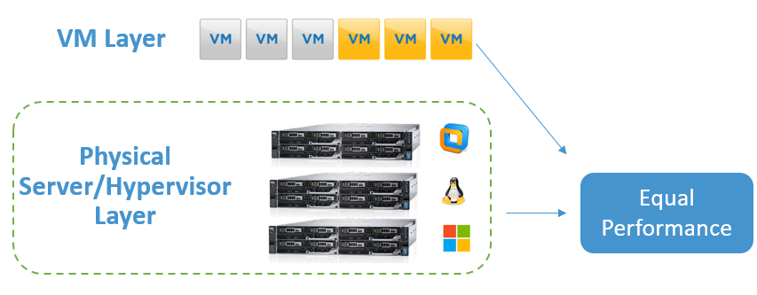
Since the Hypervisor approach gets all the performance, but the performance will be shown in one aggregated graph, the Guest VM Performance data points that are collected through the telemetry file retrieval are useful in determining the highest performing VMs in the working set.

In a separate activity and a separate project, one could target those top-tier VMs directly with the Live Optics collector to get a deep scan view of those selected Virtual Machines and the applications they might be running.

Note: The Live Optics collector understands the difference between Hypervisors in a VSAN configuration vs. a traditional external storage-supported scenario. The Collector will dynamically switch APIs when a VSAN supported scenario is encountered to focus on ONLY Front-End Capacity and IOPS. This will appropriately isolate the real workload from the overhead generated by the VSAN provider.

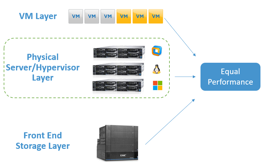
Storage Layer

While the first two might be obvious now that it is been pointed out, this last layer introduces a near-religious debate. However, it is relatively straightforward. Like the relationship between VMs and their Hypervisor, Storage arrays are also not going to produce a workload unless a Server initiates the task.

Assuming you have five servers communicating to a storage array, they are doing so through a fabric that eventually communicates to the storage controllers.

This is creating a gating activity like cars on a highway that must go through a toll plaza. Each of the 5 servers are sending down IO activity to the storage array and we would see a similar effect on Storage Front End IOPS as a result of the controller being the aggregation point.

This means that the Live Optics approach safely simulates and predicts the Front End IOPS of a storage array, without needing to communicate with the storage array itself.

Front-End Server IOPS = Front-End Storage IOPS

The Live Optics Viewer allows you to selectively opt in or opt-out internal server drives if you wanted to isolate IO and capacity, and then recalculate the project. This can be used to target a specific storage provider and get more precise details. 

Sizing projects when migrating to HCI

When sizing the migration of Virtual Machines, Live Optics recommends that you take Performance requirements from the Hypervisors that are supporting them for at least 24 hours.

4 hours of performance is the bare minimum to understand any real impact of performance over time.

24 hours show you the impact of the backup cycles or if one does not appear to exist.

Sizing projects when migrating storage appliances

If your servers are staying and the project is to only upgrade the storage array, the performance can also be taken from the hosts and it is recommended that you also use a 24-hour performance window.

In this scenario you might have physical Windows, Linux, and VMware and other OSes. Live Optics supports a heterogeneous blend of OSes in a single collection for this reason.

Effects on Public Cloud conversations

There is a compelling set of proof that the concepts in this document are real as they pertain to the net benefit of workloads running against shared resources.

If this were not true, the technologies such as CI, HCI, VSAN, and even virtualized storage arrays could not be effective and would not exist.

So, while we must accommodate sizing projects correctly, it is not necessary or to advise considering workloads by itself.

Coincidentally, this does play into Public Cloud consideration. Each instance of a VM is billed independently in the public cloud against its CPU consumption, Memory consumption, Capacity, and Performance.

The net result of this is that the cost benefits of moving to a highly virtualized environment can be erased when moving even low-performing VMs to a public cloud, as the net aggregation benefit covered in this document would not be in your favor.

If you have any questions, please reach out to Live Optics Support at liveoptics.support@dell.com.