
Deep Learning with Dell EMC Isilon

Oct 19, 2026
Deep Learning with Dell EMC Isilon ​This document demonstrates how the Dell EMC Isilon F800 All-Flash Scale-out NAS and Dell EMC PowerEdge C4140 with NVIDIA Tesla V100 GPUs can be used to accelerate and scale deep learning training workloads.

Executive summary

Overview

Deep learning techniques have enabled great success in many fields such as computer vision, natural language processing (NLP), gaming and autonomous driving by enabling a model to learn from existing data and then to make corresponding predictions. The success is due to a combination of improved algorithms, access to large datasets and increased computational power. To be effective at enterprise scale, the computational intensity of deep learning neural network training requires highly powerful and efficient parallel architectures. The choice and design of the system components, carefully selected and tuned for deep learning use-cases, can make the difference in the business outcomes of applying deep learning techniques. The Dell EMC Isilon F800 All-Flash Scale-out NAS, along with Dell EMC C4140 PowerEdge Servers and NVIDIA Volta Graphic Processing Units (GPUs) have been demonstrated to deliver excellent performance results in industry-standard deep learning benchmarks.

Audience

This document is intended for organizations interested in simplifying and accelerating deep learning solutions with advanced computing and scale-out data management solutions. Solution architects, system administrators and others interested readers within those organizations constitute the target audience.

Revisions

Date

Description

August 2018

Initial release

April 2019

Added information about Isilon tiering and RAPIDS

November 2021

Updated template

Introduction

Introduction

Deep learning is an exciting area of machine learning using simulated neural networks to enable accurate pattern recognition of complex real-world patterns by computers. These new levels of innovation have applicability across nearly every industry vertical.  Some of the early adopters include advanced research, precision medicine, high tech manufacturing, advanced driver assistance systems (ADAS) and autonomous driving.  The demand for even greater deep learning performance is driving the development of advanced deep learning software frameworks, massively parallel compute in the form of Graphic Processing Units (GPUs) for embarrassingly parallel model training, and scale-out file systems to support the concurrency and Petabyte scale of the unstructured image and video data sets.

This document demonstrates how the Isilon F800 and NVIDIA GPUs along with PowerEdge C4140 Servers can be used to architect artificial intelligence solutions that accelerate and scale deep learning workloads. The results of multiple industry-standard image classification benchmarks using TensorFlow are included.

Isilon storage for deep learning

Isilon storage for deep learning

Dell EMC Isilon F800 represents the 6th generation of hardware built to run the well-proven and massively scalable OneFS operating system. Each F800 chassis contains four storage nodes with 60 high-performance Solid State Drives (SSDs) and eight (8) 40 Gigabit Ethernet network connections. OneFS combines up to 144 nodes in 36 chassis into a single high-performance file system designed to handle the most intense I/O workloads such as deep learning. As performance and capacity demands increase, both can be scaled-out simply and non-disruptively, allowing applications and users to continue working.
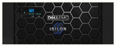
Figure 1.   Dell EMC Isilon F800

Dell EMC Isilon F800 has the following features.

  • Low latency, high throughput, and massively parallel IO for AI.
  • Up to 250,000 file IOPS per chassis, up to 9 Million IOPS per cluster
  • Up to 15 GB/s throughput per chassis, up to 540 GB/s per cluster
  • 96 TB to 924 TB raw flash capacity per chassis; up to 33 PB per cluster (All-Flash)

This shortens time for training and testing analytical models on for data sets from 10’s TBs to 10’s of PBs on AI platforms such as TensorFlow, SparkML, Caffe, or proprietary AI platforms.

  • The ability to run AI in-place on data using multi-protocol access.
  • Multi-protocol support such as SMB, NFS, HTTP and native HDFS to maximize operational flexibility

This eliminates the need to migrate/copy data and results over to a separate AI stack. Organizations can perform Deep Learning and run other IT apps on same data already on Isilon by adding F800 nodes to existing cluster.

  • Enterprise grade features out-of-box.
  • Enterprise data protection and resiliency
  • Robust security options

This enables organizations to manage AI data lifecycle with minimal cost and risk, while protecting data and meeting regulatory requirements.

  • Extreme scale 
  • Seamlessly tier between All Flash, Hybrid and Archive nodes via SmartPools.
  • Grow-as-you-go scalability with up to 33 PB capacity per cluster
  • Up to 36 chassis (144 nodes) may be connected to form a single cluster with a single namespace and a single coherent cache
  • Up to 85% storage efficiency to reduce costs

Organizations can achieve AI at scale in a cost-effective manner, enabling them to handle multi-petabyte data sets with high resolution content without re-architecture and/or performance degradation.

There are several key features of Isilon OneFS that make it an excellent storage system for deep learning workloads that require performance, concurrency, and scale. These features are detailed below.

OneFS caching

The OneFS caching infrastructure design is predicated on aggregating the cache present on each node in a cluster into one globally accessible pool of memory. This allows all the nodes’ memory cache to be available to every node in the cluster. Remote memory is accessed over an internal interconnect and has much lower latency than accessing hard disk drives.

The OneFS caching subsystem is coherent across the cluster. This means that if the same content exists in the private caches of multiple nodes, this cached data is consistent across all instances. 

OneFS uses up to three levels of read cache, plus an NVRAM-backed write cache, or coalescer. These, and their high-level interaction, are illustrated in the following diagram
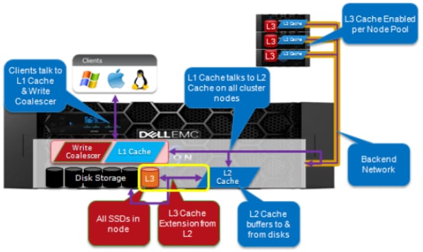
Figure 2.   OneFS caching architecture

This feature enables fast iterative analytics where the data is alternately ready from and written to disk.

File reads

For files marked with an access pattern of concurrent or streaming, OneFS can take advantage of pre-fetching of data based on heuristics used by the Isilon SmartRead component. SmartRead can create a data pipeline from L2 cache, prefetching into a local L1 cache on the captain node. This greatly improves sequential-read performance across all protocols and means that reads come directly from RAM within milliseconds. For high-sequential cases, SmartRead can very aggressively prefetch ahead, allowing reads or writes of individual files at very high data rates.

SmartRead intelligent caching allows for very high read performance with high levels of concurrent access. Importantly, it is faster for Node 1 to get file data from the cache of Node 2 (over the low-latency cluster interconnect) than to access its own local disk. SmartRead algorithms control how aggressive the pre-fetching is (disabling pre-fetch for random-access cases) and how long data stays in the cache, and optimizes where data is cached.
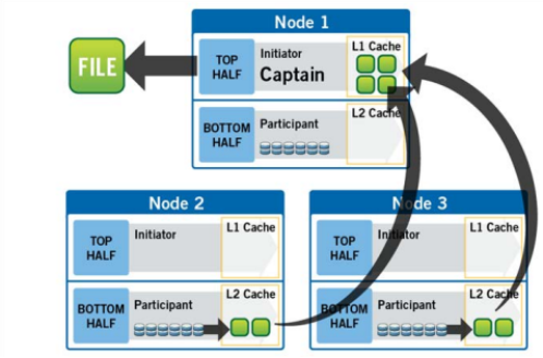
Figure 3.   A file read operation on a 3-node Isilon cluster

Locks and concurrency

OneFS has a fully distributed lock manager that marshals locks on data across all nodes in a storage cluster. The locking manager is highly extensible. It allows for multiple lock personalities to support both file system locks as well as cluster-coherent protocol-level locks such as SMB share mode locks or NFS advisory-mode locks. OneFS also has support for delegated locks such as CIFS oplocks and NFSv4 delegations. Every node in a cluster is a coordinator for locking resources and a coordinator is assigned to lockable resources based upon an advanced hashing algorithm. 

For more detailed technical overview of Isilon OneFS, refer to https://www.emc.com/collateral/hardware/white-papers/h10719-isilon-onefs-technical-overview-wp.pdf.

Efficient locking is critical to support the efficient parallel IO profile demanded by deep learning workloads enabling currency up into the millions. 

Storage tiering

Dell EMC Isilon SmartPools software enables multiple levels of performance, protection, and storage density to co-exist within the same file system. The software unlocks the ability to aggregate and consolidate a wide range of applications within a single extensible, ubiquitous storage resource pool. This helps provide granular performance optimization, workflow isolation, higher utilization, and independent scalability – all with a single point of management.

SmartPools allows you to define the value of the data within your workflows based on policies, and automatically aligns data to the appropriate price/performance tier over time. Data movement is seamless, and with file-level granularity and control via automated policies, manual control, or API interface, you can tune performance and layout, storage tier alignment, and protection settings – all with minimal impact to your end-users.

Storage tiering has a very convincing value proposition, namely separating data according to its business value, and aligning it with the appropriate class of storage and levels of performance and protection. Information Lifecycle Management techniques have been around for a number of years, but have typically suffered from the following inefficiencies: complex to install and manage, involves changes to the file system, requires the use of stub files, etc.

Dell EMC Isilon SmartPools is a next generation approach to tiering that facilitates the management of heterogeneous clusters. The SmartPools capability is native to the Isilon OneFS scale-out file system, which allows for unprecedented flexibility, granularity, and ease of management. In order to achieve this, SmartPools leverages many of the components and attributes of OneFS, including data layout and mobility, protection, performance, scheduling, and impact management.

A typical Isilon cluster will store multiple datasets with different performance, protection, and price requirements. Generally, files that have been recently created and accessed should be stored in a hot tier while files that have not been accessed recently should be stored in a cold (or colder) tier. Because Isilon supports tiering based on a file’s access time, this can be performed automatically. For storage administrators that want more control, complex rules can be defined to set the storage tier based on a file’s path, size, or other attributes.

All files on Isilon are always immediately accessible (read and write) regardless of their storage tier and even while being moved between tiers. The file system path to a file is not changed by tiering. Storage tiering policies are applied, and files are moved by the Isilon SmartPools job, which runs daily at 22:00 by default.

For more details, see Storage Tiering with Dell EMC Isilon SmartPools.

Deep learning training performance and analysis

Introduction

In this section, the performance of deep learning training is measured using TensorFlow. The well-known ILSVRC2012 dataset (often referred to as ImageNet) was used for benchmarking performance. This dataset contains 1,281,167 training images in 144.8 GB. (All unit prefixes use the SI standard—base 10—where 1 GB is 1 billion bytes.) All images are grouped into 1000 categories or classes. This dataset is commonly used by deep learning researchers for benchmarking and comparison studies.

Since the entire ILSVRC2012 dataset is only 144.8 GB and can easily fit into system memory, the size of the dataset was increased 10 times to properly exercise the storage system (Isilon F800).  We did this by applying 10 random data augmentation techniques to each JPEG image in the dataset. This is standard practice in data analytics and deep learning to increase size of data sets. The augmented images were then converted to a TensorFlow TFRecords database. In total, this “10x” dataset contained 12,811,670 JPEG images in 1,448 GB split across 1024 files. The average JPEG image size is 113 KB, and the average TFRecord file size is 1.41 GB.

TFRecords file format is a Protocol Buffers binary format that combines multiple raw image files together with their metadata into one binary file. It maintains the image compression offered by the JPEG format and the total size of the dataset remained the same.

The benchmark utilized in this document uses this data to train two different convolutional neural network (CNN) models that are popular for image classification – ResNet50 and AlexNet. ResNet50 is much more accurate but it requires a lot more computation. Although neither of these are state-of-the-art today, knowing their performance can be useful when evaluating different hardware and software platforms.

Hardware configuration

The hardware comprises of a cluster with a head node, compute nodes, Isilon storage, and networks. The head node roles can include deploying the cluster of compute nodes, managing the compute nodes, user logins and access, providing a compilation environment, and job submissions to compute nodes. The compute nodes are the work horse and execute the submitted jobs.  Software from Bright Computing called Bright Cluster Manager is used to deploy and manage the whole cluster.

Figure 4 shows the high-level overview of the cluster which includes one PowerEdge 740 head node, n PowerEdge C4140 compute nodes, each with 4 NVIDIA Tesla V100 GPU’s, 1 chassis of Isilon F800 storage, and two networks. All compute nodes are interconnected through an InfiniBand switch. All compute nodes and the head node are also connected to a 1 Gigabit Ethernet management switch which is used by Bright Cluster Manager to administer the cluster. An Isilon storage solution is dual connected to the FDR-40GigE Gateway switch so that it can be accessed by the head node and all compute nodes.

Horovod, a distributed TensorFlow framework, was used to scale the training across multiple compute nodes.

Refer to Appendix B: Benchmark setup and execution for further configuration details.
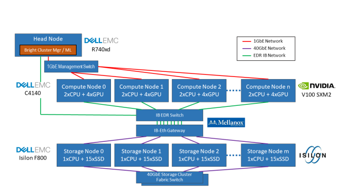
Figure 4.   Overview of the cluster

Benchmark results

The results of the benchmarks are summarized in the charts below.
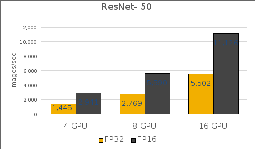
(a) Resnet50
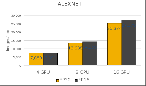
(b) AlexNet

Figure 5.   Training throughput benchmark results

Detailed performance analysis

To better understand the load on the storage subsystem, the Isilon performance was profiled using Isilon InsightIQ while training the model. In Figure 6, only two compute nodes are performing training (AlexNet, FP16, 1.448 TB dataset). There is an aggregate read throughput of 12 Gbits/sec (1500 MB/sec) and the Isilon front-end network traffic is split evenly between two Isilon nodes. Disk throughput also starts at around 12 Gbits/sec (1500 MB/sec), but it is split evenly between all four Isilon nodes. Additionally, the disk throughput decreases simply because more of the data is coming from Isilon’s cache. For these benchmarks, the cache was cleared before each run and a real-world 1.448 TB data set was used to guarantee the data set couldn’t be cached in-memory on Isilon to ensure a valid load on the disk.  The Isilon cluster was configured with 4 nodes with 256 GB RAM each).  Note: The 1024 files are read in random order (but sequentially within each file) so some files can be served from cache if they were accessed recently.
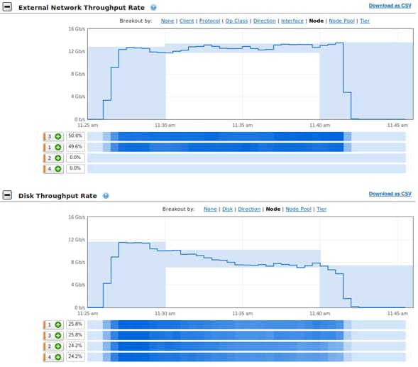
Figure 6.   InsightIQ metrics during training of AlexNet, 2 compute nodes, FP16, 1.448 TB dataset

The preceding figure shows the CPU, memory, and GPU utilization on one compute node (with 4 GPU’s), and the network and disk throughput on a single Isilon chassis (4 nodes) when running Resnet50 FP16 training with the 1.448 TB dataset. The training speed is steady at 2941 images/sec throughout the duration of training.

The CPU utilization on the C4140 compute nodes is around 33% out of 40 cores, which are used for file I/O, TFRecords parsing, JPEG decoding, distorting, and cropping.

Only around 19% of 384 GiB of memory on the C4140 compute nodes are used. The Linux buffer (page cache) on the compute server usage increases while it caches the TFRecord files until all of the RAM is used. Although the entire 1.448 TB dataset cannot be cached in the compute node, the 1024 files are read in random order (but sequentially with each file) so some files can be served from the Linux page cache if they were accessed recently. 

The network and Isilon are fast enough to feed data to GPUs to keep them at high utilization and to keep the training speed at 2,941 images/sec. The average GPU utilization was around 95% across the four GPUs. This high GPU utilization indicates the system was architected (CPU, memory, network, Isilon, etc.) to avoid any IO bottlenecks.
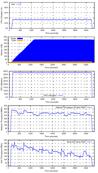
Figure 7.   CPU utilization, memory usage and GPU utilization on one compute node, and network and disk throughput on Isilon when running Resnet50 with the 1.448 TB dataset

Floating point precision (FP16 vs. FP32)

The NVIDIA V100 GPU contains a new type of processing core called Tensor Cores which support mixed precision training. Although many High Performance Computing (HPC) applications require high precision computation with FP32 (32-bit floating point) or FP64 (64-bit floating point), deep learning researchers have found they are able to achieve the same inference accuracy with FP16 (16-bit floating point) as can be had with FP32. In this document, mixed precision training which includes FP16 and FP32 representations is denoted as “FP16” training.

In experiments where training tests were executed using FP16 precision, the batch size was doubled since FP16 consumes only half the memory for floating points as FP32. Doubling the batch size with FP16 ensures that GPU memory is utilized equally for both types of tests.

Although FP16 makes training faster, it requires extra work in the neural network model implementation to match the accuracy achieved with FP32. This is because some neural networks require their gradient values to be shifted into FP16 representable range, and they may do some scaling and normalization to use FP16 during training. For more details, please refer to NVIDIA mixed precision training.

Dataset preprocessing pipeline optimizations

The training performance of the tested neural networks are affected by various flags in the benchmark. It was found that the training performance of Resnet50 could be improved by changing the default value of the flag datasets_num_private_threads to 4. This setting allows image preprocessing, which includes TFRecord parsing, JPEG decoding, distorting, and cropping, to be performed by multiple threads concurrently. The performance comparison between the baseline version and this tuned version for Resnet50 is shown in the following figure. There was no obvious performance improvement for AlexNet. With one compute node (4 GPUs), the performance was improved from 2,657 images/sec to 2,941 images/sec. With two compute nodes (8 GPUs), the performance was improved from 4,560 images/sec to 5,590 images/sec.
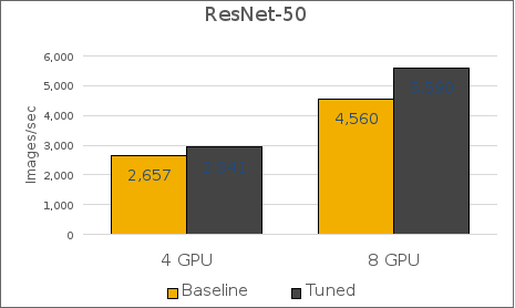
Figure 8.   Performance comparison of Resnet50 between the baseline and tuned (datasets_num_private_threads=4) versions

Storage profile of deep learning training

The storage I/O profile of the training benchmark is relatively simple. From the perspective of the storage subsystem, a 1.41 GB TFRecord file is opened and read sequentially in its entirety from beginning to end. Multiple TFRecord files are read concurrently. The order in which files are opened is effectively random. As measured using the Linux lsof (list open files) command, a four-GPU compute node reads 120 files concurrently (30 files per GPU). Four such compute nodes would read 480 files concurrently.

If the images/sec throughput is known, the required storage throughput can be calculated easily by multiplying by the average image size of 113 KB. For instance, 1000 images/sec * 113 KB/image = 113 MB/sec. Of course, this does not account for caching at the compute nodes or Isilon nodes which would reduce the required disk throughput.

Another aspect that should be considered when designing deep learning infrastructure is the generation of the TFRecord files. Although this is not part of the TensorFlow CNN benchmark results, it is a very I/O intensive operation and it must be performed before training can begin. To generate the TFRecord files, the directories with the individual JPEG images are listed, file names are ordered randomly, and then multiple processes read these JPEG files while writing TFRecord files. This can be effectively parallelized across multiple compute nodes with MPI or other parallel computing frameworks.

Performance-based sizing considerations

Deep Learning workloads vary significantly with respect to the demand for compute, memory, disk, and IO profiles, often by orders of magnitude. Sizing guidance for the GPU quantity and configuration of Isilon nodes can only be provided when these resource requirements are known in advance. That said, it’s usually beneficial to have a few data points on ratio of GPU count per Isilon node for common Image Classification benchmarks.

The following table shows a few such data points: 

Table 1.      Sizing consideration based on benchmarked workloads

Storage performance demanded

Benchmark

Required storage throughput per V100 GPU (MB/sec/GPU)

V100 GPUs per Isilon F800 node

Low

ResNet50, fp32

40

60

Medium

ResNet50, fp16

80

30

High

AlexNet

200

13

To illustrate, in the above example, ResNet50 with floating point precision of FP16 with 16 GPUs will need a storage system that can read 16 * 80 = 1280 MB/sec. As another example, ResNet50 with FP16 on 120 GPUs would require 4 Isilon F800 nodes (1 chassis).

The above data points were generated using the hardware configuration specified in Appendix A: Hardware and software for training the models (and NOT for inferencing); they do not account for node failure, drive failure, network failure, administrative jobs, or any other concurrent workloads supported by Isilon. Actual ratio of number of GPUs per Isilon node will vary from the above data points based on several factors:

  • Hardware configuration might be different from what is specified in Appendix A: Hardware and software based on compute, memory, disk, and IO profile requirements.
  • Deep Learning algorithms are diverse and don’t necessarily have the same infrastructure demands as the benchmarks listed above.
  • Characteristics and size of the data sets will be different from the data sets described in this whitepaper and used to generate the above data points.
  • Inferencing workloads will alter the compute and IO requirement significantly from training workloads.
  • Accounting for node/drive/network failures, admin jobs or other workloads accessing Isilon simultaneously.

An understanding of the IO throughput demanded per GPU for the specific workload and the total storage capacity requirements can help provide better guidance on Isilon node count and configuration. It is recommended to reach out to the Isilon account and SME teams to provide this guidance for the specific deep learning workload, throughput, and storage requirements.

Machine Learning with RAPIDS

Machine Learning with RAPIDS

The RAPIDS suite of software libraries can accelerate some machine learning algorithms and analytics pipelines. Like TensorFlow, it uses NVIDIA GPUs for acceleration. RAPIDS requires CUDA 9.2 or 10.0 so you must ensure that the NVIDIA driver on the host supports this.

The following steps show how to run a simple RAPIDS benchmark using the mortgage demo.

mkdir -p /mnt/isilon/data/mortgage

cd /mnt/isilon/data/mortgage 

# Use below for a quick test with 1 year of data.

wget http://rapidsai-data.s3-website.us-east-2.amazonaws.com/notebook-mortgage-data/mortgage_2000.tgz

tar -xzvf mortgage_2000.tgz

# Use below for the full benchmark with 17 years of data.

wget http://rapidsai-data.s3-website.us-east-2.amazonaws.com/notebook-mortgage-data/mortgage_2000-2016.tgz

tar -xzvf mortgage_2000-2016.tgz 

docker run --runtime=nvidia \

-it \

-p 8888:8888 \

-p 8787:8787 \

-p 8786:8786 \

-v /mnt:/mnt \

--name rapidsai \

nvcr.io/nvidia/rapidsai/rapidsai:0.5-cuda10.0-runtime-ubuntu18.04-gcc7-py3.7

jupyter@12b8e8800eef:/rapids/notebooks$

source activate rapids

(rapids) jupyter@12b8e8800eef:/rapids/notebooks$

bash utils/start-jupyter.sh

  1. Open your browser to http://host:8888/.
  2. Open the notebook mortgage/E2E.ipynb.
  3. Change acq_data_path to "/mnt/isilon/data/mortgage/acq". Change other paths in same way.
  4. For a quick test, change end_year to 2000 and part_count to 1. For a benchmark, leave these at the default of 2016 and 16.
  5. From the menu, click Kernel -> Restart Kernel and Run All Cells.
  6. Record the time elapsed for following cells:
  • ETL (cell 17)
  • Load into GPUs (cell 21)
  • Training (cell 22)

Conclusion

Conclusion

This document discussed key features of Isilon that make it a powerful persistent storage for Deep Learning solutions.  We presented a typical hardware architecture for deep learning by combining Dell EMC C4140 servers with embedded NVIDIA Volta GPUs and all-flash Isilon storage. We ran several image classification benchmarks and reported system performance based on the rate of images processed and throughput profile of IO to disk. We also monitored and reported the CPU, GPU utilization, and memory statistics that demonstrated that the server, GPU, and memory resources were fully utilized while IO was not fully saturated.

Deep Learning algorithms have a diverse set of requirements with various compute, memory, IO, and disk capacity profiles. That said, the architecture and the performance data points presented in this whitepaper can be utilized as the starting point for building deep learning solutions tailored to varied set of resource requirements. More importantly, all the components of this architecture are linearly scalable and can be expanded to provide deep learning solutions that can manage 10s of PBs of data.

While the solution presented here provides several performance data points and speaks to the effectiveness of Isilon in handling large scale Deep Learning workloads, there are several other operational benefits of persisting data for deep learning on Isilon:

  • The ability to run AI in-place on data using multi-protocol access.
  • Enterprise grade features out-of-box.
  • Seamlessly tier to higher density nodes for cost-effective scaling

In summary, Isilon based Deep Learning solutions deliver the capacity, performance, and high concurrency to eliminate the I/O storage bottlenecks for AI.  This provides a solid foundation for large scale, enterprise-grade deep learning solutions with a future proof scale-out architecture that meets your AI needs of today and scales for the future. 

Appendix A: Hardware and software

Overview

The system used to perform the benchmarking is bundled together as the Dell EMC Ready Solution for AI. It is described in detail in this section.

Table 2.      Hardware and software in test bed

Hardware—head node 
Cluster head node PowerEdge R740xd

CPU 

2 x Intel Xeon 6148 @ 2.4GHz 

Memory 

384GB DDR4 @ 2667MT/s

Hardware—compute node

Cluster compute node

PowerEdge C4140

Number of compute nodes

4

CPU

2 x Intel Xeon 6148 @ 2.4GHz

Memory

384GB DDR4 @ 2667MT/s

Disks

2x M.2, 240GB in Raid1 

GPU

V100-SXM2

Software and firmware

Operating System

Red Hat Enterprise Linux 7.4

Linux Kernel

3.10.0-693.el7.x86_64

BIOS

1.1.6

CUDA compiler and GPU driver

CUDA 9.1.85 (390.46)

Python

2.7.5

Deep learning datasets

Dataset for training

ILSVRC2012 training dataset, 1,281,167 images

Deep learning libraries and frameworks

CUDNN

7.0

NCCL

2.1.15

Horovod

0.12.1

TensorFlow

1.8

Compute node configuration

Deep learning methods would not have gained success without the computational power to drive the iterative training process. Therefore, a key component of deep learning solutions is highly capable nodes that can support compute intensive workloads. The state-of-art neural network models in deep learning have more than 100 layers which require the computation to be able to scale across many compute nodes in order for any timely results. The Dell EMC PowerEdge C4140, an accelerator-optimized, high density 1U rack server, is used as the compute node unit in this solution. The PowerEdge C4140 can support four NVIDIA Volta SMX2 GPUs, both the V100-SXM2 as well as the V100-PCIe models. The following figure shows the CPU-GPU and GPU-GPU connection topology of a compute node.
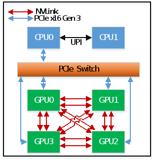
Figure 9.   Topology of a compute node

GPU

The NVIDIA Tesla V100 is the latest data center GPU available to accelerate Deep Learning. Powered by NVIDIA Volta, the latest GPU architecture, Tesla V100 GPUs enable data scientists, researchers, and engineers to tackle challenges that were once difficult.  With 640 Tensor Cores, Tesla V100 is the first GPU to break the 100 teraflops (TFLOPS) barrier of deep learning performance. 

Table 3.      V100-SXM2 specifications

Description

Value

CUDA Cores

5120

GPU Max Clock Rate (MHz)

1530

Tensor Cores

640

Memory Bandwidth (GB/s)

900

NVLink Bandwidth (GB/s) (uni-direction)

300

Deep Learning (Tensor OPS)

120

TDP (Watts)

300

With the V100-SXM2 model, all GPUs are connected by NVIDIA NVLink. V100-SXM2 GPUs provide six NVLinks per GPU for bi-directional communication. The bandwidth of each NVLink is 25GB/s in uni-direction and all four GPUs within a node can communicate at the same time, therefore the theoretical peak bandwidth is 6*25*4=600GB/s in bi-direction.

Network

The solution comprises of three network fabrics. The head node and all compute nodes are connected with a 1 Gigabit Ethernet fabric. This connection is primarily used by Bright Cluster Manager for deployment, maintenance and monitoring the solution.

The second fabric connects the head node, and all compute nodes are through 100 Gb/s EDR InfiniBand. The EDR InfiniBand switch is the Mellanox SB7800 which has 36 ports. This fabric is used for IPC by the applications as well as to serve NFS from Isilon.

The third switch in the solution is the gateway switch and connects the Isilon F800 to the head node and compute nodes. Isilon’s external interfaces are 40 Gigabit Ethernet. Hence, a switch which can serve as the gateway between the 40GbE Ethernet and InfiniBand networks is needed for connectivity to the head and compute nodes. The Mellanox SX6036 is used for this purpose. The gateway is connected to the InfiniBand EDR switch and the Isilon.

Isilon

The following Isilon hardware was used for the benchmarking in this document.

Table 4.       Specification of tested Isilon F800

Item

Description

Model

Isilon F800-4U-Single-256GB-1x1GE-2x40GE SFP+-48TB SSD

Number of Nodes

4

Number of Chassis

1

Processors Per Chassis

4 x Intel Xeon Processor E5-2697A v4

Raw Capacity Per Chassis

192 TB (60 x 3.2 TB SSD)

Throughput Per Chassis

Up to 15 GB/s

Front-End Networking

2 x 40GbE (QSFP+) per node

Infrastructure Networking

2 x InfiniBand QDR per node

Storage Type

SSD

Number of Chassis Possible

36

OneFS version

8.1.0.2

Note: The Isilon cluster used to validate this solution used InfiniBand for the back-end (infrastructure) networking. However, it is recommended that new Isilon deployments use 40GbE for the back-end networking, even for deep learning workloads.

Isilon configuration

The default and minimal configuration of Isilon is sufficient for excellent performance of the deep learning workloads tested in this document.

In a minimal configuration, there will be a single Isilon chassis containing four Isilon F800 nodes. Each Isilon node should have at least one 40 Gigabit Ethernet port connected to a front-end switch. In most situations, this will provide as much bandwidth as can be provided by the F800. However, for protection from switch failures, the 2nd 40 Gigabit Ethernet port should also be connected.

Mounting to Isilon

When NFS clients establish a mount to an Isilon cluster, the recommended best practice is to mount to a DNS name which the Isilon cluster will resolve to one of its IP addresses. These IP addresses are automatically assigned and reassigned to individual Isilon nodes to handle load balancing and node failures. This method of mounting is simple to administer since the mount host is the same for all nodes (e.g. isilon.example.com). However, when there are just a few high-throughput clients, one Isilon node may have significantly more client connections than others, leading to an imbalance and reducing performance. To prevent this problem, each client can be mounted to a different fixed IP address to force a good balance. For instance, compute node 1 connects to Isilon node 1, compute node 2 connects to Isilon node 2, etc. Note that although a specific client node connects to only a single Isilon node, an I/O request will typically involve the disks and caches in all nodes of the Isilon cluster.

If archive-class Isilon nodes are part of the Isilon cluster, it is recommended that NFS clients do not connect to them as their slower CPUs will reduce client performance. Even if the dataset is known to be stored on the archive-class nodes, it is recommended to access them via the F800 all-flash nodes with faster CPU and more RAM. In general, archive-class nodes do not need to be assigned front-end IP addresses as all I/O to them will go through the back-end network.

Configuring automatic storage tiering

This section explains one method of configuring storage tiering for a typical DL workload. The various parameters should be changed according to the expected workload.

  1. Build an Isilon cluster with two or more node types. For example, F800 all-flash nodes for a hot tier and H500 hybrid nodes for a cold tier.
  2. Obtain and install the Isilon SmartPools license.
  3. Enable Isilon access time tracking with a precision of 1 day. In the web administration interface, click File System -> File System Settings. Alternatively, enter the following in the Isilon CLI:

isilon-1# sysctl efs.bam.atime_enabled=1
isilon-1# sysctl efs.bam.atime_grace_period=86400000

  1. Create a tier named hot-tier that includes the F800 node pool. Create a tier named cold-tier that includes the H500 node pool.
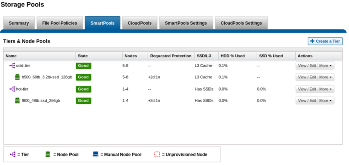
Graphical user interface

Description automatically generated

  1. Edit the default file pool policy to change the storage target to hot-tier. This will ensure that all files are placed on the F800 nodes unless another file pool policy applies that overrides the storage target.
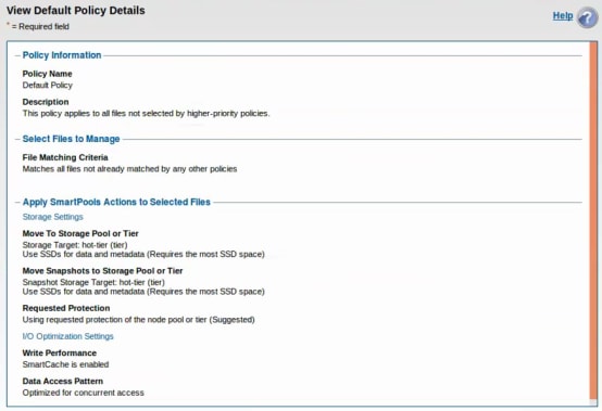
  1. Create a new file pool policy to move all files that have not been accessed for 30 days to the H500 (cold) tier.
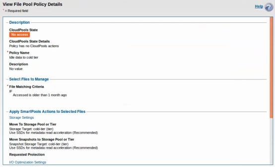
Configuration is now complete. To test this configuration, follow these steps:

  1. Start the Isilon SmartPools job and wait for it to complete. This will apply the above file pool policy and move all files to the F800 nodes (assuming that all files have been accessed within the last 30 days).

isilon-1# isi job jobs start SmartPools
isilon-1# isi status

  1. Use the isi get command to confirm that a file is stored in the hot tier. Note that first number in each element of the inode list (1, 2, and 3 below) is the Isilon node number that contains blocks of the file. For example:

isilon-1# isi get -D /ifs/data/imagenet-scratch/tfrecords/train-00000-of-01024
* IFS inode: [ 1,0,1606656:512, 2,2,1372672:512, 3,0,1338880:512 ]
*  Disk pools:         policy hot-tier(5) -> data target f800_48tb-ssd_256gb:2(2), metadata target f800_48tb-ssd_256gb:2(2)

  1. Use the ls command to view the access time.

isilon-1# ls -lu /ifs/data/imagenet-scratch/tfrecords/train-00000-of-01024
-rwx------    1 1000  1000  762460160 Jan 16 19:32 train-00000-of-01024

  1. Instead of waiting for 30 days, you may manually update the access time of the files using the touch command.

isilon-1# touch -a -d '2018-01-01T00:00:00' /ifs/data/imagenet-scratch/tfrecords/*
isilon-1# ls -lu /ifs/data/imagenet-scratch/tfrecords/train-00000-of-01024
-rwx------    1 1000  1000  762460160 Jan  1  2018 train-00000-of-01024

  1. Start the Isilon SmartPools job and wait for it to complete. This will apply the above file pool policy and move the files to the H500 nodes. Record the number of bytes moved and the duration.

isilon-1# isi job jobs start SmartPools
isilon-1# isi status

  1. Use the isi get command to confirm that the file is stored in the cold tier. 

isilon-1# isi get -D /ifs/data/imagenet-scratch/tfrecords/train-00000-of-01024
* IFS inode: [ 4,0,1061376:512, 5,1,1145344:512, 6,3,914944:512 ]
*  Disk pools:         policy cold-tier(9) -> data target h500_60tb_3.2tb-ssd_128gb:15(15), metadata target h500_60tb_3.2tb-ssd_128gb:15(15)

  1. Run the training benchmark as described in the previous section. Be sure to run at least 4 epochs so that all TFRecords are accessed. Monitor the Isilon cluster to ensure that disk activity occurs only on the H500 nodes. Note that since the files will be read, this will update the access time to the current time. When the SmartPools job runs next, these files will be moved back to the F800 tier. By default, the SmartPool job runs daily at 22:00.

  2. Start the Isilon SmartPools job and wait for it to complete. This will apply the above file pool policy and move the files to the F800 nodes.

isilon-1# isi job jobs start SmartPools
isilon-1# isi status

  1. Use the isi get command to confirm that the file is stored in the hot tier.

isilon-1# isi get -D /ifs/data/imagenet-scratch/tfrecords/train-00000-of-01024
* IFS inode: [ 1,0,1606656:512, 2,2,1372672:512, 3,0,1338880:512 ]
*  Disk pools:         policy hot-tier(5) -> data target f800_48tb-ssd_256gb:2(2), metadata target f800_48tb-ssd_256gb:2(2)

Appendix B: Benchmark setup and execution

Appendix B: Benchmark setup and execution

The procedure to download the dataset and build the TFRecord files is documented at https://github.com/tensorflow/models/tree/master/research/inception#getting-started. The repository for the benchmark used is https://github.com/alsrgv/benchmarks which has optimizations and required fixes when using Horovod to distribute training with TensorFlow. The hash of the commit used is 3b90c14, dated May 31, 2018. The CNN benchmark scripts in scripts/tf_cnn_benchmarks were used.

Before running any benchmark, the cache on the compute nodes were cleared with the command “sync; echo 3 > /proc/sys/vm/drop_caches”. Additionally, all caches on all Isilon nodes were cleared with “isi_for_array isi_flush”.

Since we use Horovod to distribute the training across multiple GPUs on multiple nodes, the mpirun command is used to run the training benchmark. Refer to https://github.com/uber/horovod/blob/8318a898a2f03fb22664ca8f5353361974f8a693/docs/benchmarks.md for details.

Below is an example command to run the training benchmark.

mpirun --allow-run-as-root --mca btl_openib_want_cuda_gdr 1 -np 16 \
python3.6 tf_cnn_benchmarks.py \
--model=resnet50 --datasets_num_private_threads=4 --distortions=False \
--variable_update=horovod --batch_size=256 --num_batches=2000 \
--data_dir=/mnt/isilon/tensorflow_10x --data_name=imagenet \
--train_dir=/mnt/Isilon/train_dir --init_learning_rate=.04 \
--use_fp16=True --use_tf_layers=False --print_training_accuracy

Below is the output from the above command. Note that many lines have been omitted for brevity. The last line shown is the training throughput in images per second.

TensorFlow:  1.8

Model:       resnet50

Dataset:     imagenet

Mode:        training

SingleSess:  False

Batch size:  4096 global

             256.0 per device

Num batches: 2000

Num epochs:  0.64

Devices:     ['horovod/gpu:0', 'horovod/gpu:1', 'horovod/gpu:2', 'horovod/gpu:3', 'horovod/gpu:4', 'horovod/gpu:5', 'horovod/gpu:6', 'horovod/gpu:7', 'horovod/gpu:8', 'horovod/gpu:9', 'horovod/gpu:10', 'horovod/gpu:11', 'horovod/gpu:12', 'horovod/gpu:13', 'horovod/gpu:14', 'horovod/gpu:15']

Data format: NCHW

Layout optimizer: False

Optimizer:   sgd

Variables:   horovod

==========

Generating model

2018-07-13 15:23:43.871841: I tensorflow/core/common_runtime/gpu/gpu_device.cc:1356] Found device 0 with properties:

name: Tesla V100-SXM2-16GB major: 7 minor: 0 memoryClockRate(GHz): 1.53

pciBusID: 0000:1e:00.0

totalMemory: 15.78GiB freeMemory: 15.34GiB

2018-07-13 15:23:44.430647: I tensorflow/core/common_runtime/gpu/gpu_device.cc:1053] Created TensorFlow device (/job:localhost/replica:0/task:0/device:GPU:0 with 14849 MB memory) -> physical GPU (device: 0, name: Tesla V100-SXM2-16GB, pci bus id: 0000:1a:00.0, compute capability: 7.0)

Step    Img/sec total_loss      top_1_accuracy  top_5_accuracy

1       2018-07-13 15:24:09 images/sec: 680.1 +/- 0.0 (jitter = 0.0)    9.788   0.000   0.004

1       2018-07-13 15:24:09 images/sec: 680.3 +/- 0.0 (jitter = 0.0)    9.003   0.000   0.004

1       2018-07-13 15:24:09 images/sec: 679.8 +/- 0.0 (jitter = 0.0)    8.518   0.000   0.000

1       2018-07-13 15:24:09 images/sec: 680.0 +/- 0.0 (jitter = 0.0)    8.386   0.000   0.000

1       2018-07-13 15:24:09 images/sec: 679.7 +/- 0.0 (jitter = 0.0)    8.585   0.000   0.008

1       2018-07-13 15:24:09 images/sec: 680.1 +/- 0.0 (jitter = 0.0)    9.207   0.000   0.000

1       2018-07-13 15:24:09 images/sec: 679.7 +/- 0.0 (jitter = 0.0)    8.530   0.000   0.000

1       2018-07-13 15:24:09 images/sec: 679.6 +/- 0.0 (jitter = 0.0)    8.213   0.000   0.008

1       2018-07-13 15:24:09 images/sec: 679.8 +/- 0.0 (jitter = 0.0)    8.494   0.000   0.004

1       2018-07-13 15:24:09 images/sec: 679.5 +/- 0.0 (jitter = 0.0)    12.650  0.008   0.008

1       2018-07-13 15:24:09 images/sec: 679.8 +/- 0.0 (jitter = 0.0)    8.375   0.000   0.008

1       2018-07-13 15:24:09 images/sec: 679.6 +/- 0.0 (jitter = 0.0)    9.301   0.008   0.016

1       2018-07-13 15:24:09 images/sec: 679.6 +/- 0.0 (jitter = 0.0)    8.332   0.000   0.000

1       2018-07-13 15:24:09 images/sec: 679.6 +/- 0.0 (jitter = 0.0)    8.275   0.000   0.000

1       2018-07-13 15:24:09 images/sec: 679.6 +/- 0.0 (jitter = 0.0)    8.658   0.000   0.000

1       2018-07-13 15:24:09 images/sec: 679.9 +/- 0.0 (jitter = 0.0)    8.506   0.000   0.008

10      2018-07-13 15:24:12 images/sec: 693.3 +/- 1.9 (jitter = 3.9)    8.147   0.000   0.004

10      2018-07-13 15:24:12 images/sec: 693.3 +/- 1.9 (jitter = 3.4)    8.227   0.000   0.000

10      2018-07-13 15:24:12 images/sec: 693.3 +/- 1.8 (jitter = 3.4)    8.294   0.000   0.000

10      2018-07-13 15:24:12 images/sec: 693.3 +/- 1.9 (jitter = 4.0)    8.398   0.000   0.000

10      2018-07-13 15:24:12 images/sec: 693.3 +/- 1.9 (jitter = 3.6)    8.351   0.000   0.008

10      2018-07-13 15:24:12 images/sec: 693.3 +/- 1.9 (jitter = 3.4)    8.270   0.000   0.000

10      2018-07-13 15:24:12 images/sec: 693.3 +/- 1.9 (jitter = 3.8)    8.273   0.000   0.012

10      2018-07-13 15:24:12 images/sec: 693.3 +/- 1.9 (jitter = 3.7)    8.142   0.000   0.004

10      2018-07-13 15:24:12 images/sec: 693.3 +/- 1.9 (jitter = 3.3)    8.361   0.000   0.000

10      2018-07-13 15:24:12 images/sec: 693.3 +/- 1.9 (jitter = 3.9)    8.293   0.000   0.004

10      2018-07-13 15:24:12 images/sec: 693.3 +/- 1.9 (jitter = 3.3)    8.165   0.000   0.004

10      2018-07-13 15:24:12 images/sec: 693.3 +/- 1.9 (jitter = 3.9)    9.824   0.000   0.000

10      2018-07-13 15:24:12 images/sec: 693.3 +/- 1.9 (jitter = 3.4)    8.171   0.000   0.000

10      2018-07-13 15:24:12 images/sec: 693.3 +/- 1.9 (jitter = 3.7)    8.413   0.004   0.008

10      2018-07-13 15:24:12 images/sec: 693.3 +/- 1.9 (jitter = 3.9)    8.116   0.000   0.000

10      2018-07-13 15:24:12 images/sec: 693.3 +/- 1.9 (jitter = 3.4)    8.146   0.000   0.004

2000    2018-07-13 15:36:25 images/sec: 695.3 +/- 0.1 (jitter = 6.0)    4.880   0.223   0.410

total images/sec: 11123.80

Appendix C: Monitoring Isilon performance

InsightIQ

To monitor and analyze the performance and file system of Isilon storage, the tool InsightIQ can be used. InsightIQ allows a user to monitor and analyze Isilon storage cluster activity using standard reports in the InsightIQ web-based application. The user can customize these reports to provide information about storage cluster hardware, software, and protocol operations. InsightIQ transforms data into visual information that highlights performance outliers, and helps users diagnose bottlenecks and optimize workflows. For more details about InsightIQ, refer to the Isilon InsightIQ User Guide.

Isilon statistics CLI

For a quick way to investigate the performance of an Isilon cluster when InsightIQ is not available, there is a wealth of statistics that are available through the Isilon CLI, which can be accessed using SSH to any Isilon node.

This first command shows the highest level of statistics. Note that units are in bytes/sec so in the example below Node 1 is sending (NetOut) 2.9 GBytes/sec to clients.

isilon-1# isi statistics system --nodes all --format top

Node   CPU   SMB FTP HTTP    NFS HDFS  Total   NetIn NetOut DiskIn DiskOut

 All 72.7%   0.0 0.0  0.0  10.0G  0.0  10.0G  304.4M  10.4G 315.4M   10.8G

   1 79.2%   0.0 0.0  0.0   2.9G  0.0   2.9G  295.0M   2.9G  70.5M    2.3G

   2 80.6%   0.0 0.0  0.0   2.7G  0.0   2.7G    3.2M   2.7G  95.5M    2.8G

   3 71.9%   0.0 0.0  0.0   2.4G  0.0   2.4G    3.4M   2.6G  75.5M    2.8G

   4 59.2%   0.0 0.0  0.0   2.0G  0.0   2.0G    2.9M   2.1G  73.9M    2.9G

The following commands shows more details related to NFS. All statistics are aggregated over all nodes.

isilon-1 # isi statistics pstat --format top
__________________________NFS3 Operations Per Second___________________________

access             2.33/s  commit             0.00/s  create             0.75/s

fsinfo             0.00/s  getattr            2.09/s  link               0.00/s

lookup             0.99/s  mkdir              0.00/s  mknod              0.00/s

noop               0.00/s  null               0.00/s  pathconf           0.00/s

read           18865.24/s  readdir            0.00/s  readdirplus        0.00/s

readlink           0.00/s  remove             0.00/s  rename             0.75/s

rmdir              0.00/s  setattr            0.00/s  statfs             0.00/s

symlink            0.00/s  write              0.75/s

Total          18872.91/s

___CPU Utilization___                                     _____OneFS Stats_____

user             1.4%                                     In         73.81 kB/s

system          72.5%                                     Out         8.96 GB/s

idle            26.1%                                     Total       8.96 GB/s

____Network Input____        ___Network Output____        ______Disk I/O_______

MB/s            12.64        MB/s          9868.11        Disk   272334.03 iops

Pkt/s       150368.20        Pkt/s      6787182.27        Read       11.73 GB/s

Errors/s         0.00        Errors/s         0.00        Write      99.63 MB/s

Appendix D: Isilon performance testing with iPerf and FIO

Introduction

iPerf is a tool for active measurements of the maximum achievable bandwidth on IP networks. It can be used to validate the throughput of the IP network path from an Isilon node to a compute node NIC. It can easily be scripted to run concurrently to allow all nodes to send or receive traffic.

FIO is a disk benchmark tool for Linux. It can be used to easily and quickly produce a storage workload that is nearly identical to the TensorFlow benchmark used in this document.

This section shows how to use iPerf and FIO.

To begin, on your head node (or first compute node), create a hosts file containing one host name (or IP address) per client. For example:

server1.example.com

server2.example.com

iPerf

Install iPerf on all compute nodes. Note that iPerf is already installed on all Isilon nodes. All versions should match.

cat hosts | xargs -i -P 0 ssh root@{} yum -y install \

iperf-2.0.4-1.el7.rf.x86_64.rpm

cat hosts | xargs -i -P 0 ssh root@{} pkill -9 iperf

cat hosts | xargs -i ssh root@{} "iperf --server --daemon > /dev/null 2>&1 &"

client_opts="-t 300 --len 65536 --parallel 2"

ssh root@isilon-1.example.com iperf -c server1.example.com ${client_opts} &

ssh root@isilon-2.example.com iperf -c server2.example.com ${client_opts} &

wait

To view the aggregate bandwidth, run the following on any Isilon node.

isi statistics system --format top --nodes all

FIO

The procedure below shows how to use FIO to benchmark NFS I/O from multiple clients concurrently.

Mount to Isilon. Each client will mount to a different Isilon IP address.

cat hosts | xargs -i -P 0 ssh root@{} mkdir -p /mnt/isilon

cat hosts | xargs -i -P 0 ssh root@{} umount /mnt/isilon

ssh root@server1.example.com mount -t nfs 10.1.1.1:/ifs \

-o rsize=524288,wsize=524288 /mnt/isilon

ssh root@server2.example.com mount -t nfs 10.1.1.2:/ifs \

-o rsize=524288,wsize=524288 /mnt/isilon

Install FIO servers.

cat hosts | xargs -i -P 0 ssh root@{} yum -y install epel-release

cat hosts | xargs -i -P 0 ssh root@{} yum -y install fio

cat hosts | xargs -i ssh root@{} fio –version

Start FIO servers.

cat hosts | xargs -i ssh root@{} pkill fio

cat hosts | xargs -i ssh root@{} fio --server --daemonize=/tmp/fio.pid

Create a FIO job file shown below, named fio1.job. Set numjobs to the number of GPUs per host. This job file performs I/O that is similar to the TensorFlow CNN benchmark. It creates 30 files per GPU and then reads them sequentially concurrently.

[global]

name=job1

directory=/mnt/isilon/tmp/fio

time_based=1

runtime=600

ramp_time=60

ioengine=libaio

numjobs=8

create_serialize=0

iodepth=32

kb_base=1000

[job1]

rw=read

nrfiles=30

size=64GiB

bs=1024KiB

direct=1

sync=0

rate_iops=83

Run the FIO job.

mkdir -p /mnt/isilon/tmp/fio

fio --client=hosts fio1.job

Appendix E: References

Appendix E: References

The following table provides links to additional references.

Table 5.      References