Deep Learning (DL) applications have become pervasive in almost every field, including application domains in science and technology. Large-scale, memory-intensive DL applications that require training of complex DL models on high-resolution data and large batch sizes result in a high amount of memory consumption during the model training phase. In such cases, often the memory being consumed exceeds the available system resources. Reliably predicting the memory consumption of a DL model being trained prior to runtime is valuable to minimize OutOfMemory errors and save limited system resources and/or computation budget (for example, when running on cloud).

In this paper, we adopt a modeling approach based on symbolic regression principles to generate an accurate memory consumption model for a DL application to predict the peak memory consumption during training. We evaluated our modeling approach using 3D U-net as an application case-study, because it exhibits high memory consumption during the training phase (close to 1TB of data for large image sizes). Based on our approach, the memory consumption model generated was able to predict the peak memory consumed during the training phase for different input size and batch sizes with less than 5% Mean Absolute Percentage Error (MAPE). We subsequently compared our model approach against models generated from other machine-learning based regression methods, demonstrating the superior accuracy of our modeling approach.

Dell Technologies and the authors of this document welcome your feedback on this document. Contact the Dell Technologies team by email.

Authors:

Sai P. Chenna, SHREC Center[1], University of Florida
Bhavesh Patel, Dell Technologies
Herman Lam, SHREC Center1, University of Florida

Note: For links to other documentation for this topic, see the Artificial Intelligence Info Hub.

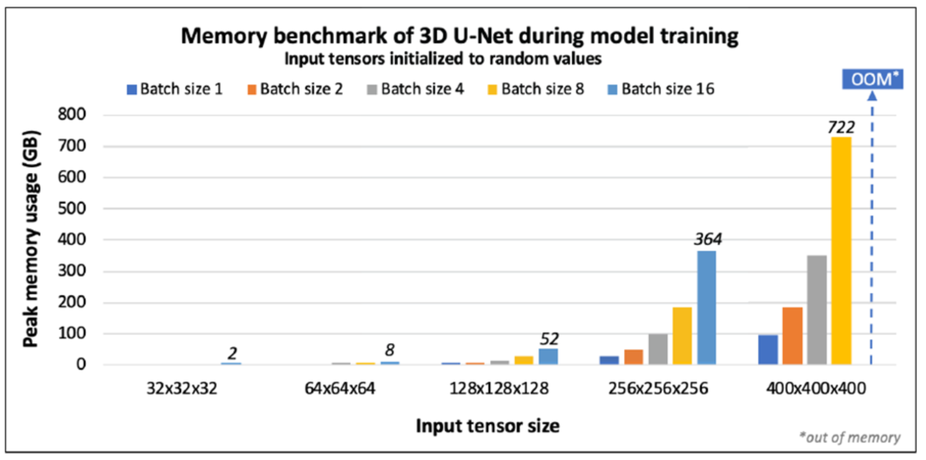
Deep Learning (DL) applications have become pervasive in application domains in various fields of science and technology [1], which have been increasingly dependent on DL methods for regression and classification tasks. Furthermore, recent advances in the computer architecture, especially with the advent of custom accelerators for Machine Learning (ML) based computations, have significantly accelerated model training and inference times. Higher model training and inference performance has led the application developers to train more complex models, and/or train on much larger training datasets in order to create better DL models. However, one common limitation in training such complex models is the high memory consumption. Depending on the network hyper-parameters such as number of layers, batch size, input data dimensions, floating point precision, and underlying framework implementation (such Tensorflow, PyTorch, and so on), memory consumption can quickly escalate beyond the capacity limitation provided by the underlying hardware. Figure 1 shows the peak memory consumed by a DL network called 3D U-net, trained to perform semantic segmentation on high resolution 3D brain MRI scans for brain tumor detection. As shown in the figure, with the increase of the input image dimensions and batch size, the peak memory consumption can quickly escalate toward and beyond 1TB, making it unfeasible to run on a single accelerator (for example, GPU) on most compute nodes.

Figure 1.   3D U-net memory consumption behavior for various input size and batch sizes during the model training phase

As mentioned previously, in memory-intensive DL workloads such as 3D U-net, the memory being consumed often exceeds the available system resources. Therefore, running the model training task without the proper knowledge on its memory requirement would result in poor utilization of the computing resources due to frequent OutOfMemory errors. In fact, a recent empirical study [2] performed to analyze the common DL workload job failures that occurred on a Microsoft Cloud platform revealed that close to 9% of the job failures are caused by OutOfMemory errors, where the jobs consume more than the available amount of memory. Due to the nature of these applications, these errors occur during the runtime, resulting in loss of valuable compute hours and a need to rerun the application with additional memory resources. Accurately estimating memory needs of memory-intensive DL workloads is therefore crucial in order to make efficient use of the underlying compute resources.

To successfully train a Deep Learning workload on a given computing resource without exceeding the memory capacity limitation, it is valuable to develop a model to estimate the peak memory consumption for a given DL network configuration. Generating a reliable memory consumption model for DL workloads has multiple advantages. Firstly, by reliably capturing the memory consumption prior to execution we can run the largest possible application configuration on the given system resources. Secondly, while scaling the model training onto multiple nodes, a common phenomenon while training large-scale DL workloads, identifying the peak memory consumption prior to runtime can help distribute the workload in an optimal manner, thereby achieving peak throughput. However, reliably predicting the memory consumption prior to runtime is a non-trivial task for application developers. As mentioned before, memory consumed during the model training phase depends on various parameters such as the network architecture, batch size, input dimension of the training data, data precision, and so on.

In this paper, we present a multi-parameter modeling approach to generate analytical models that accurately predicts the peak memory consumption of a Deep Learning workload. In the next section, we present a DL application, 3D U-net as our case study. First, we perform a memory characterization of 3D U-net, identifying key parameters that contribute to its high memory consumption. As a baseline, we then generate a basic analytical model by studying the network architecture to estimate memory requirements. We will show how a model generated by studying the network architecture falls short of accurately predicting the runtime memory consumption, thereby highlighting a need for a better modeling approach for generating a memory consumption model.

In the section Modeling methodology we present our modeling approach, which leverages symbolic regression principles [5] to generate a multi-parameter model capturing the impact of key application parameters on memory consumption. As shown in Model evaluation, using a small number of training samples from the 3D U-net case study, our modeling approach was able to generate memory consumption models that produced predictions that are less than 5% Mean Absolute Percentage Error (MAPE) when validated against untrained data points. We also compared our model approach against models generated from other machine-learning based regression methods, demonstrating the superior accuracy of our modeling approach.

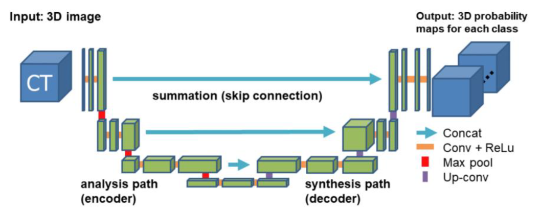
Figure 2.   3D U-Net architecture.

3D U-nets are typically used in medical imaging for processing three-dimensional volumetric data [3]. 3D U-net has a typical encoder-decoder structure where the encoder structure analyses the input image and performs dimensionality reduction. The decoder path performs up-convolution to produce full image segmentation. Both encoder and decoder paths involve 3D convolutions, max pooling layers, and batch normalizations. Figure 2 shows our 3D U-net architecture. By design, 3D U-net is a symmetric network, meaning the model can be trained and inferred with different image sizes. Due to the high-resolution, three-dimensional images being used for training, and the network hyper-parameters being specified (such as batch size, filter dimensions, and number of layers), memory consumption can quickly escalate beyond the capacity of the underlying hardware, as shown in Figure 1.

To understand the memory consumption behavior of, and develop a baseline memory consumption model for, 3D-net, we first identified the key contributors that dominate most of the memory consumption. The two main memory objects that dominate most of the memory consumption during the model training phase are (i) intermediate tensors (activation maps), and (ii) model weights. Activation maps are the tensors generated after the subsequent convolution and max pooling layers. The size of these tensors depends on four key parameters:

• input image dimension
• batch size
• number of filters
• number of layers

During the forward pass operation in the model training phase, we generate multiple activation maps for each image specified in the batch size. As a result, memory consumption by activation maps scales linearly with the batch size. Equation 1 specifies the memory consumed in bytes due to activation maps:

• H,W,D define height, width, and depth of the input training images, respectively
• Cin and Cout denotes the number of input and output channels
• Fk denotes the number of filters in the first layer
• bz specifies the training batch size

Figure 3.   Equation 1

Another key contributor for memory consumption is model parameters. Unlike activation maps, memory consumed by model parameters is fixed for a given network and does not depend on the input image dimensions and batch sizes. The total number of model parameters that include both model weights and biases depend on (i) number of filters, (ii) filter dimensions of convolution and concatenation layers, and (iii) number of layers. Equation 2 specifies the memory consumed in bytes by the model weights for the 3D U-net architecture specified in Figure 1:

• Kh* Kw * Kd denotes the filter dimensions of the convolution layers
• Kh1* Kw1 * Kd1 denotes the filter dimensions of the concatenation layers
• Kh11* Kw11 * Kd11 denotes the filter dimension of the output layer

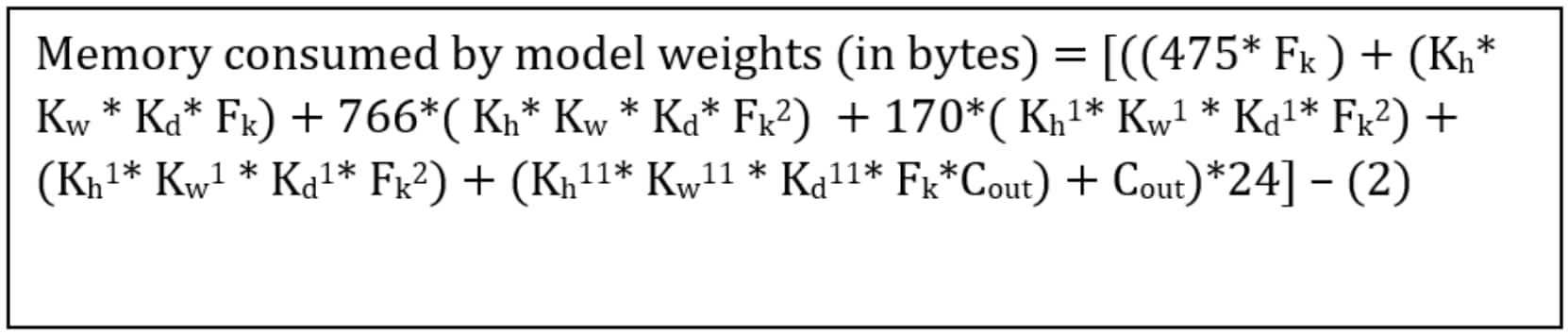
Figure 4.   Equation 2

Figure 5.   Evaluation of memory consumption model for 3D U-net developed by studying the intermediate tensors and model parameters.

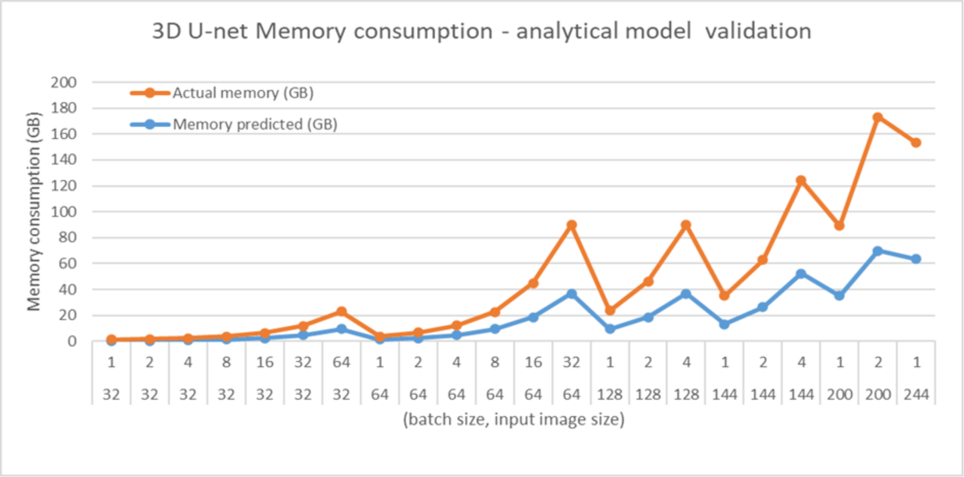
Figure 5 shows the memory consumption predictions made from the baseline analytical models specified in Equations 1 and 2 and the corresponding measured data acquired through memory profiling. The analytical model combines the memory consumed by the activation maps and model weights to predict the peak memory consumption. As shown in the figure, while the analytical model was able to capture the trend in terms of the memory consumption with regard to input image dimension and batch size, the model was not able to predict the peak memory consumption accurately during the training phase. Specifically, for larger input image sizes, where the memory consumption escalates to hundreds of gigabytes, the analytical model (which was generated by studying the intermediate tensors and model parameters) falls significantly short in predicting the actual peak runtime memory performance. This example demonstrates a practical disadvantage of the pure analytical modeling approach, which requires detailed knowledge of the application and the targeted architecture being modeled. Even with expert knowledge, the resulting model often deviates from actual execution due to machine and tool specific behaviors that are difficult to predict or understand.

In the next section, we present an empirical multi-parameter modeling approach to generate accurate memory consumption models by leveraging symbolic regression principles [4].

Symbolic regression is an approach that searches the space of all possible mathematical equations to find an equation that minimizes some error metric for a given set of training data. Like other machine-learning regression approaches, the goal of symbolic regression is to leverage training data to build a model that generalizes well to test data. Although studied for several decades [5-7], symbolic regression has limited usage due to numerous challenges compared to other regression techniques. Most significantly, symbolic regression has an infinitely large search space due to the existence of infinite equations. In fact, not only is the search space infinite, but there are an infinite number of equations that coincide with any set of training data. As a result, the goal of symbolic regression is often not merely to find the equation with the least error, but also the simplest equation that minimizes the error, because a simpler equation tends to generalize better by minimizing overtraining.

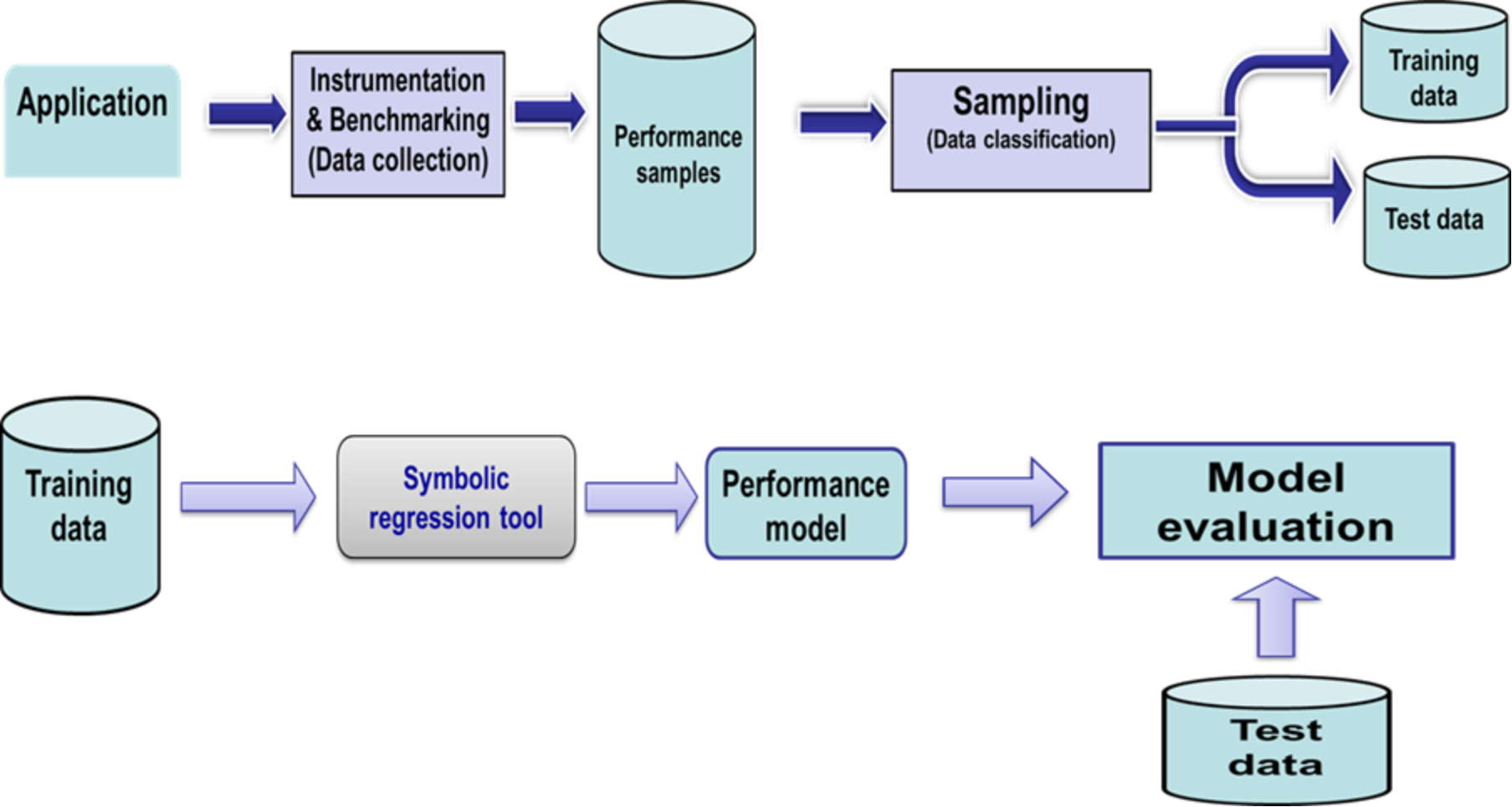
Figure 6.   Multi-parameter modeling workflow using symbolic regression

Figure 6 shows our modeling workflow. To generate the performance models, we begin by collecting the performance samples by instrumenting the application under consideration and benchmarking the application for various performance parameters to collect the performance samples (Step 1 in Figure 6). The performance metric under consideration could be execution time, total number of FLOPs, or in this case, peak memory consumption during execution. Upon collecting the performance samples, the data is classified into training data and test data through sampling (Step 2). The training data is used during model generation process. For the model generation in our study, we use Pandora [8], a symbolic regression based tool built in Python. The tool leverages several data structures and algorithms from the DEAP evolutionary algorithm library [9], which were extended with numerous optimizations for symbolic regression. While the original developers developed Pandora for the approximate computing applications [8], we leveraged the framework for performance and peak memory consumption modeling. In a previous work, we performed extensive evaluation on Pandora for performance modeling by building accurate coarse-grained multi-parameter models for various HPC applications [4]. More details about the Pandora tool are given in Pandora – symbolic regression based modeling tool. When the performance model has been generated, the next step in the workflow is to use the test/validation data to evaluate the accuracy of our model (Step 4). In Model evaluation, we demonstrate the accuracy of our modeling approach by generating a memory consumption model of 3D U-net to predict the peak memory consumption during the training phase.

The Pandora tool [8] was developed initially for the purposing of approximate computing – to provide inexpensive solutions for complex computing tasks within a reasonable amount of error tolerance. By combing through various mathematical possibilities to arrive at the same solution through empirical modeling, the tool can be used for many regression/curve-fitting tasks. Previous work involved using Pandora for compiler optimization – exploring different approximations for sequential code containing loop carried dependencies [8].

In addition to approximation computing, Pandora has been customized for application and architecture performance modelling [4]. In particular, Pandora provides the three desirable characteristics that are crucial for performance modeling of large-scale systems:

• domain-agnostic
• true multi-parameter modeling
• feasible model generation time

Domain-agnostic is a desirable property so the approach can be applicable to a wider range of applications and systems. Detailed knowledge of the application and target system being modeled is not required. Also, in most cases, the performance of an application or system sub-component to be modeled can have multiple parameters that affect its performance. Hence, the modeling approach should not be restricted to a limited number of parameters to generate an accurate performance model. Finally, the model generation times should be fast enough for iterative refinement if necessary.

In our previous work [4], we performed a systematic study to evaluate the accuracy of the performance models generated using Pandora for various High-Performance Computing (HPC) applications. In that study, it was shown that multi-parameter modeling using symbolic regression (Pandora) was able to generate accurate models with less than 8% MAPE, while using relatively fewer training samples as compared to other machine-learning based regression methods. In this paper, we use Pandora to generate a memory consumption model for 3D U-net application. We validate our model by comparing the predicted results against the measured peak memory performance (test data) of the application. Subsequently, we perform a comparative evaluation of the symbolic regression approach with other prominent ML based regression methods for memory consumption modeling.

Model generation process

In this sub-section, we briefly describe how Pandora generates an analytical model by leveraging symbolic regression principles. While there are multiple strategies to perform symbolic regression, Pandora makes use of genetic programming [5,10,11], not to be confused with more general genetic algorithms. Genetic programming imitates the processes of evolution to develop a solution to a problem. For the purposes of symbolic regression, genetic programming defines genes consisting of mathematical primitives. These primitives are generally basic, low-level operations (such as add, multiply, and so on) but can potentially be arbitrarily complex operations. Figure 7 shows the steps involved in the model generation process. Genetic programming initially creates a population of individuals, which for symbolic regression consists of random equations built from the defined primitives. Genetic programming then evolves different solutions over a number of generations, where each generation involves crossover/reproduction and mutation [5, 12]. Before the end of each generation, a selection process (analogous to natural selection) removes a percentage of individuals from the population based on a pre-defined fitness function. This process generally iterates for either a pre-defined number of generations, or until there is a lack of improvements for a number of generations.

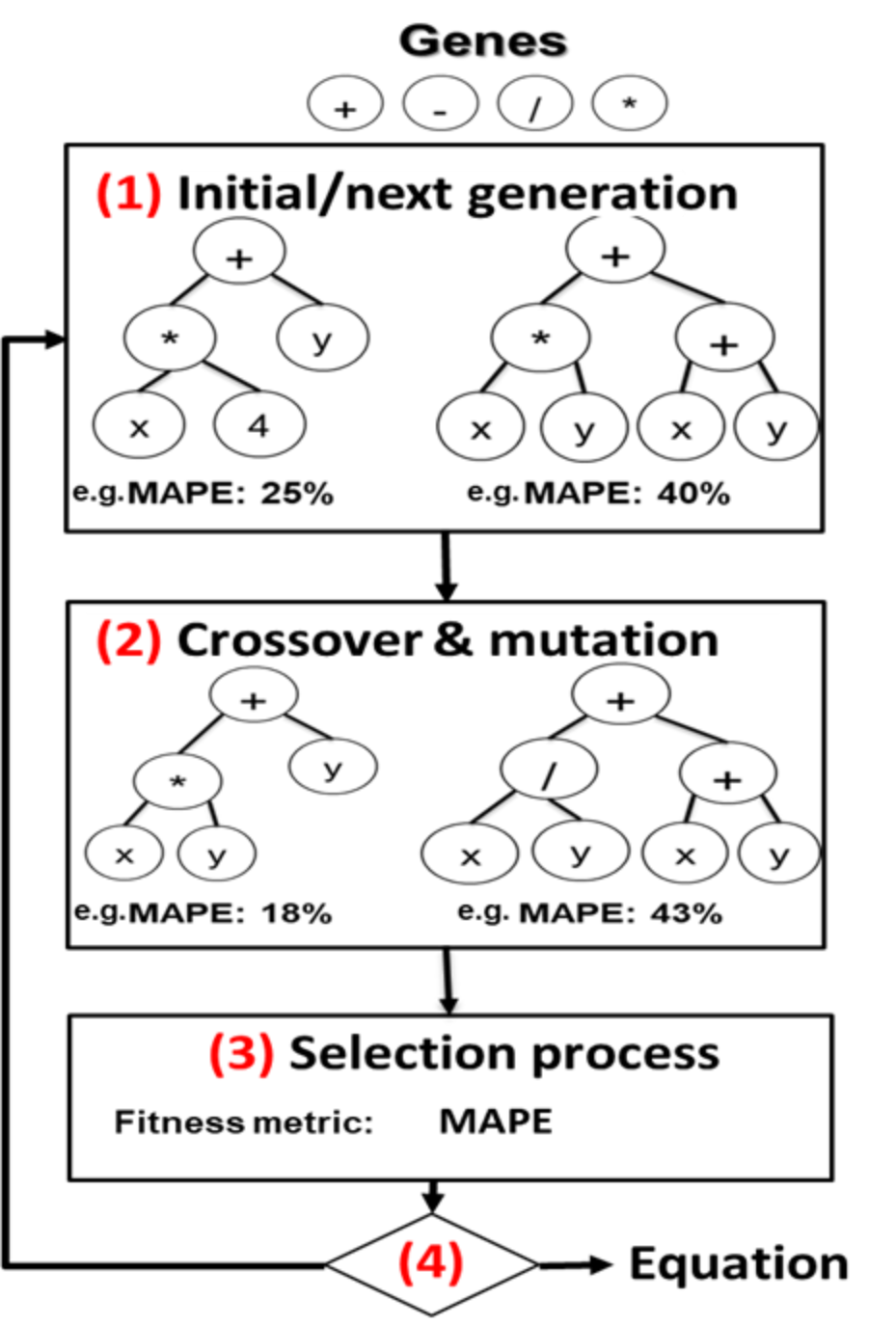
Figure 7.   Model generation process in Pandora

Genetic programming is guided by a provided fitness function that specifies desirable characteristics of an individual. For symbolic regression, the most basic fitness function is an error metric. For situations where simple equations are preferable, the function can also include the size, computational complexity, and so on, of the equation. Although any error metric can be used for symbolic regression, common examples include root mean-squared error (RMSE), mean-squared error (MSE), and mean absolute-percentage error (MAPE). Because we are using symbolic regression to generate peak memory consumption models, we will use MAPE, which is useful for showing how closely a set of test/training data fits the regression model.

To perform symbolic regression, we provide Pandora with a configuration file that specifies a number of genetic-programming parameters: training data, test data, primitives/genes, mutation probability, crossover probability, fitness function, population size, and number of generations. Although domain knowledge can be used to fine-tune the configuration file, in our experiments we used the same configuration for all experiments to provide a lower bound on the quality of the results, and to demonstrate that symbolic regression can perform well even without any deep knowledge of the application or architecture being modeled. Our memory consumption model was built using primitives consisting of addition and multiplication. We also included square and cube as primitives, because we expected these to be common in our memory consumption model. Although symbolic regression can generally discover square and cube operations with multiply primitives, inclusion of the square and cube primitive can reduce training times. We have eliminated other basic arithmetic primitives such as subtraction and division because it is not natural for them to be in the memory consumption model.

For all experiments, we used a plus-selection evolutionary algorithm [12], which considers both the parents and offspring during selection. The selection algorithm used a double tournament method [13], with a parsimony size of 1.1 and a fitness size of 3. We used five different mutation operators [9] that the tool selected randomly for each mutation. We used a one-point crossover operator. The mutation probability for each individual was 50%. Crossover probability was 100%. For all examples, we used a population size of 300 with 150 total generations. We empirically determined these values to work well for most symbolic-regression problems we have evaluated. A complete tradeoff exploration of all genetic-programming parameters is outside the scope of this study, but has been studied extensively in evolutionary-algorithm studies [14]. To optimize constants, we used the Levenberg–Marquardt non-linear least squares algorithm [15]. Upon completion, the tool outputs the resulting equation and then tests that equation against the provided test data to determine the resulting generalization error.

In this section, we evaluate our modeling approach on the 3D U-net case study to generate an analytical peak memory consumption model. In Experimental setup, the experimental setup, data collection, and sampling processing employed to generate the training and test data are described. In Model validation, the evaluation of the model generated by Pandora is presented, comparing the result against the validation data. Finally in Comparative evaluation with ML regression methods, we compare our modeling approach with other machine-learning based approaches that have proven to be promising candidates for performance modeling [16].

To generate the memory consumption model for 3D U-net, we first begin by collecting performance samples by running the 3D U-net model training for various image dimensions and batch sizes. The memory profiler mprof was used to profile the memory consumption during the training phase, and the peak memory consumed was extracted during execution (Step 1 in Figure 6). Intel’s optimized Tensorflow version 2.4 was used, and the application was written in Keras (version 2.2.3). More details about the software stack and the hardware utilized to collect the performance samples are described in the reproducibility section in the Appendix.

To facilitate the data collection for various input dimensions and batch sizes, we have generated scripts that create random input data for the desired image dimensions. The synthetic input data is used for the model training. The memory consumption was sampled throughout execution using the mprof profiler (Step 2 in Figure 6). Mprof polls the program to collect the memory consumption details at a sampling interval (default is 0.1 seconds). When the training is complete, we extract the peak memory consumed as our performance sample for that run. Table 1 shows the parameter space used for collecting performance samples.

Table 1.      Parameter design space used for memory consumption modeling for 3D U-net

When all the performance samples have been collected, we randomly classify the data into training data and test data (Step 2). 70% of the total collected samples was used for training and the remaining 30% for test/validation data. Random sampling is used to eliminate any bias in training data and to help generate a model that can generalize well to the test data.

The training data was inputted into the Pandora symbolic regression tool to generate the memory consumption model (Step 3 in Figure 6). The performance metric under consideration is the peak memory consumption during execution, and the input parameters are the image dimension and batch size of the 3D U-net. The configuration parameters used for model generation are those discussed in Model generation process.

Figure 8 shows the accuracy of our generated model compared to the validation data (that is, the 30% test data from benchmarking). We use Mean Absolute Percentage Error (MAPE) as our evaluation metric. As you can see, the predicted memory consumption results (from the Pandora symbolic regression tool) for the various image dimension/batch sizes match closely to the measured data. On average, the model had a MAPE of 4.15%. Compared to results generated by the base analytical model in Case-study application: 3D U-Net and Figure 5, the performance model generated through symbolic regression performed significantly better.

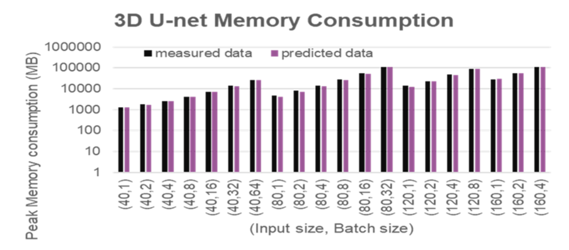
Figure 8.   3D U-net memory consumption model (symbolic regression) evaluation

Over the last decade, machine-learning based regression methods have been widely deployed in multiple fields for regression and classification tasks. Recent advances in computer architecture have made it possible to train complex machine learning regression models on large datasets. While these regression models have been actively used for fields such as weather forecasting, e-commerce, and finance, not much progress has been made in the performance modeling domain. Malakar et al. [16] performed a detailed study on the efficiency of the machine learning regression methods for performance modeling of scientific applications. They evaluated multiple machine learning regression methods, ranging from simple multi-variate linear regression to instance-based methods such as nearest-neighbor regression [17], kernel-based methods [18], decision tree based methods [19] such as random forests, and, deep learning neural networks. Based on their evaluation on multiple Mantevo [20] HPC benchmarks, they determined that complex ML methods such as bagging, boosting, and Deep Neural Network models performed well while generating accurate performance models for HPC applications.

In this paper, we perform a comparative evaluation of our symbolic regression based approach with these ML regression methods. Based on the work described by Malakar et. al [16], we have selected XGBoost (xgb), random forest (rfr), extremely randomized trees (ert), and Deep Neural Networks (dnn) for memory consumption modeling. For this study, the Python Scikit library package was used to build the ML regression models. Using the MinMaxScaler transformation, normalization on the training data was performed as a part of the data pre-processing. For all the decision tree methods, the default values were used, and the number of trees set to 1000. As with symbolic regression, configuration parameters play a significant role in the model generation process, but a detailed study on the impact of configuration parameters on the model performance is out of scope for this paper. However, for consistency, the configuration parameters were set to default for all the ML regression methods. For Deep Neural Networks, the Keras library was used to build the network that runs on top of Tensorflow. We used a three-layer feed forward network with dropout layers in between. Finally, an Adam optimizer was used and the models were trained for 100 epochs.

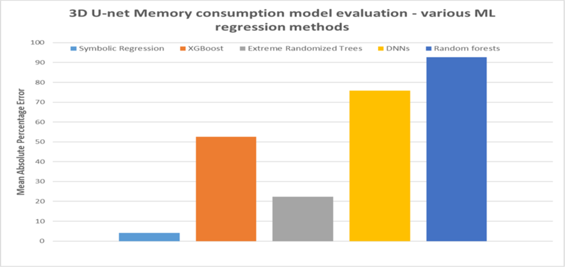
Figure 9 compares the accuracy of the model generated by symbolic regression with the selected ML regression methods. As shown in the figure, the symbolic regression model performed significantly better than the other ML methods using the same performance samples. The symbolic regression model has a MAPE of 4.15%, whereas ert, rfr, xgb, and dnn have a MAPE of 22.35%, 92.75%, 52.56%, and 75.91%, respectively.

Again, the results shown in Figure 9 is based on using the same performance samples for all the modeling methods. If we vary the size and other characteristics of the sampled data, the results may not be the same. Detailed study on the impact of varying different sampling and model parameters on the model performance is outside the scope of this paper. Interested readers are referred to such extensive comparison in our earlier study, the results of which are consistent with the results shown in Figure 9. In that earlier study, we applied the symbolic regression modeling approach to develop performance models for a petascale HPC application called CMT-nek [24] and two HPC mini-apps (Cloverleaf [22] and LULESH [23]) which capture the key computation patterns in many real-world scientific applications. We also showcase the ability of our modeling approach to determine the true function accurately by using a set of synthetic test functions. In our findings, we observed that, in general, symbolic regression performed significantly better than other ML regression techniques for a given number of performance samples. We also varied the size of the performance samples and observed that on average, increasing the performance samples for training improved the model accuracy for the other ML regression methods, but at the cost of longer training time. And, at some point, some of the ML based regression methods may equal or outperform symbolic regression. However, as we stated in Pandora – symbolic regression based modeling tool, one of the three desirable characteristics that are crucial for performance modeling of large-scale systems is feasible model generation time. In general, we observed that with a limited number of performance samples, our symbolic regression-based modeling approach was able to generate the most accurate models.

Figure 9.   Comparison of accuracies of various memory consumption models generated using symbolic regression and other ML based regression methods

Deep Learning applications have been growing in scale and complexity over the last few years due to significant breakthroughs in algorithms and system architecture. As a result, there has been a growing demand for using high resolution data on complex Deep Learning networks for model training. This has resulted in high memory consumption during the model training phase, often beyond the system limitation.It has therefore become important for application users to reliably predict the memory consumption requirements before starting the model training process.

In this paper, we present a multi-parameter modeling approach to accurately generate a memory consumption model. By reliably predicting the memory requirements of a model prior to runtime, we would be able to optimize the workload distribution without exceeding the system memory requirements. Also, while scaling the model training onto multiple nodes, identifying the peak memory consumption prior to runtime can help distribute the workload in an optimal manner, and achieve peak throughput. We evaluated our modeling approach on a 3D U-net deep learning application and generated a memory consumption model for the network. We subsequently validated the accuracy of our model by predicting the peak memory consumption on some untrained data points and achieved a Mean Absolute Percentage Error of 4.15%. Finally, a comparative evaluation was performed with other machine-learning based regression techniques and confirmed that the symbolic regression approach does a better job at generating accurate models for the 3D U-net peak memory consumption, in the presence of a limited set of performance samples. Going forward, we would like to extend our modeling approach to predict the runtime performance of other large-scale DL workloads.

[1] Y. LeCun, Y. Bengio, and G. Hinton. 2015. Deep learning. Nature 521, 7553 (2015), 436–444

[2] Ru Zhang, Wencong Xiao, Hongyu Zhang, Yu Liu, Haoxiang Lin, and Mao Yang. 2020. An Empirical Study on Program Failures of Deep Learning Jobs. In Proceedings of the 42nd International Conference on Software Engineering (Seoul, Republic of Korea) (ICSE ’20). Association for Computing Machinery, NY, USA, 1159–1170.

[3] Çiçek, Özgün, et al. "3D U-Net: learning dense volumetric segmentation from sparse annotation." International conference on medical image computing and computer-assisted intervention. Springer, Cham, 2016.

[4] Chenna, Sai P., Greg Stitt, and Herman Lam. "Multi-parameter performance modeling using symbolic regression." 2019 International Conference on High Performance Computing & Simulation (HPCS). IEEE, 2019.

[5] J. R. Koza, Genetic Programming II: Automatic Discovery of Reusable Programs. Cambridge, MA, USA: MIT Press, 1994.

[6] J. McDermott, D. R. White, S. Luke, L. Manzoni, M. Castelli, L. Vanneschi, W. Jaskowski, K. Krawiec, R. Harper, K. De Jong, and U.-M. O’Reilly, “Genetic programming needs better benchmarks,” in Proceedings of the 14th Annual Conference on Genetic and Evolutionary Computation, ser. GECCO ’12. New York, NY, USA: ACM, 2012, pp. 791–798. [Online]. Available: http://doi.acm.org/10.1145/2330163.2330273.

[7] M. Schmidt and H. Lipson, “Distilling free-form natural laws from experimental data,” Science, vol. 324, no. 5923, pp. 81–85, 2009. [Online]. Available: http://science.sciencemag.org/content/324/5923/81.

[8] Stitt, Greg, and David Campbell. "PANDORA: An Architecture-Independent Parallelizing Approximation-Discovery Framework." ACM Transactions on Embedded Computing Systems (TECS) 19.5 (2020): 1-17.

[9] F.-A. Fortin, F.-M. De Rainville, M.-A. Gardner, M. Parizeau, and C. Gagné, “DEAP: Evolutionary algorithms made easy,” Journal of Machine Learning Research, vol. 13, pp. 2171–2175, jul 2012.

[10] D. P. Searson, D. E. Leahy, and M. J. Willis, “Gptips: An open source genetic programming toolbox for multigene symbolic regression.”

[11] G. S. Hornby, “ALPS: The age-layered population structure for reducing the problem of premature convergence,” in Proceedings of the 8th Annual Conference on Genetic and Evolutionary Computation, ser. GECCO ’06. New York, NY, USA: ACM, 2006, pp. 815–822. [Online]. Available: http://doi.acm.org/10.1145/1143997.1144142.

[12] H.-G. Beyer and H.-P. Schwefel, “Evolution strategies – a comprehensive introduction,” Natural Computing, vol. 1, no. 1, pp. 3–52, Mar 2002. [Online]. Available: https://doi.org/10.1023/A:1015059928466.

[13] S. Luke and L. Panait, “Fighting bloat with nonparametric parsimony pressure,” in Parallel Problem Solving from Nature — PPSN VII, J. J. M. Guervós, P. Adamidis, H.-G. Beyer, H.-P. Schwefel, and J.-L. Fernández-Villacañas, Eds. Berlin, Heidelberg: Springer Berlin Heidelberg, 2002, pp. 411–421.

[14] F. G. Lobo, C. F. Lima, and Z. Michalewicz, Parameter Setting in Evolutionary Algorithms, 1st ed. Springer Publishing Company, Incorporated, 2007.

[15] M. Kommenda, G. Kronberger, S. Winkler, M. Affenzeller, and S. Wagner, “Effects of constant optimization by nonlinear least squares minimization in symbolic regression,” in Proceedings of the 15th Annual Conference Companion on Genetic and Evolutionary Computation, ser. GECCO ’13 Companion. New York, NY, USA: ACM, 2013, pp. 1121–1128. [Online]. Available: http://doi.acm.org/10.1145/2464576.2482691.

[16] Malakar, Preeti, et al. "Benchmarking machine learning methods for performance modeling of scientific applications." 2018 IEEE/ACM Performance Modeling, Benchmarking and Simulation of High Performance Computer Systems (PMBS). IEEE, 2018.

[17] C. M. Bishop and N. M. Nasrabadi, Pattern recognition and machine learning. Springer, 2006, vol. 4, no. 4.

[18] A. J. Smola and B. Schölkopf, “A tutorial on support vector regression,” Statistics and computing, vol. 14, no. 3, pp. 199–222, 2004.

[19] W.-Y. Loh, “Classification and regression trees,” Wiley interdisciplinary reviews: data mining and knowledge discovery, vol. 1, no. 1, pp. 14–23, 2011.

[20] M. A. Heroux, D. W. Doerfler, P. S. Crozier, J. M. Willenbring, H. C. Edwards, A. Williams, M. Rajan, E. R. Keiter, H. K. Thornquist, and R. W. Numrich, “Improving Performance via Mini-applications,” Sandia National Laboratories, Tech. Rep. SAND2009-5574, 2009.

[21] Chenna, Sai P., et al. "Scalable Performance Prediction of Irregular Workloads in Multi-Phase Particle-in-Cell Applications." 2021 IEEE International Parallel and Distributed Processing Symposium Workshops (IPDPSW). IEEE, 2021.

[22] M. A. Heroux, D. W. Doerfler, P. S. Crozier, J. M. Willenbring, H. C. Edwards, A. Williams, M. Rajan, E. R. Keiter, H. K. Thornquist, and R. W. Numrich, “Improving Performance via Mini-applications,” Sandia National Laboratories, Tech. Rep. SAND2009-5574, 2009.

[23] I. Karlin, J. Keasler, and R. Neely, “Lulesh 2.0 updates and changes,” Tech. Rep. LLNL-TR-641973, August 2013.

[24] Banerjee, Tania, et al. "Cmt-bone—a proxy application for compressible multiphase turbulent flows." 2016 IEEE 23rd International Conference on High Performance Computing (HiPC). IEEE, 2016.